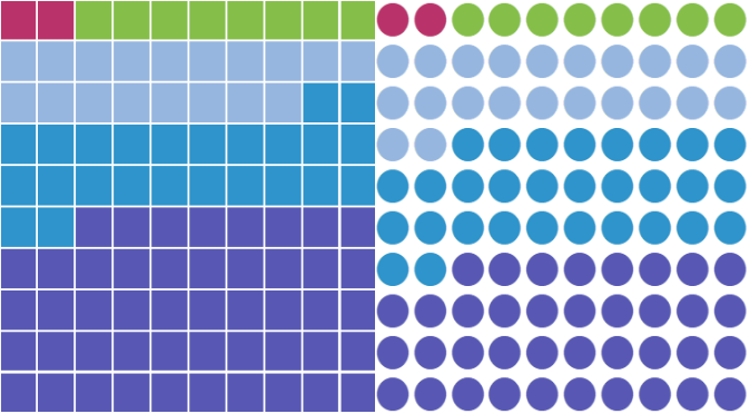
Ok, don’t eat the waffle chart
In a previous post, I discussed making a Button Bar Chart. That whole process really inspired me to think about simplified charts for presentations.
Which got me thinking about Waffle Charts.
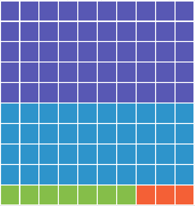
Waffle charts are excellent for looking at data sets where the smallest numbers are the important ones. You can use colour (as I have above) to make those numbers stand out.
But oddly, I don’t see people using a lot of waffle charts in their presentations. And there is no template for a waffle chart in Excel.
You can find some interesting ideas about building Excel waffle charts for dashboard purposes and I recommend this article to you: Interactive Waffle Charts in Excel
However, I was looking for something different. Something that wouldn’t have me counting and colouring cells manually (shudder).
Building the Waffle
I chose to build the waffle chart using a series of conditional formatting rules. The first step was creating the formula to count the cells of the waffle.
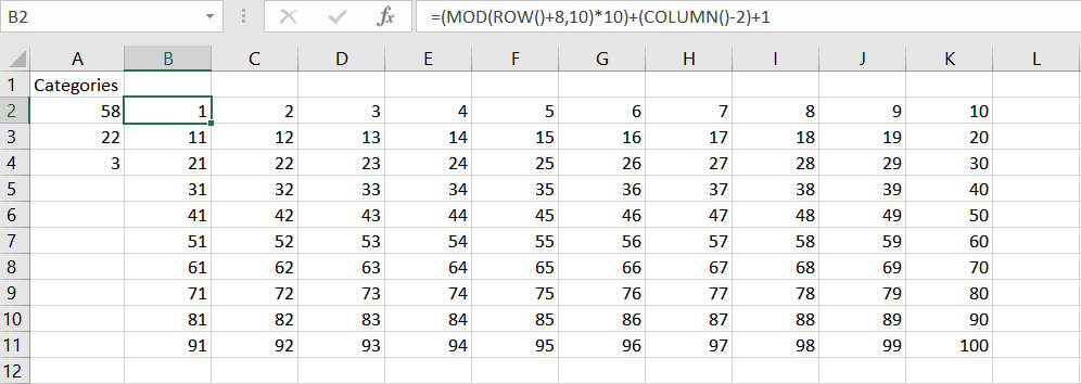
In case the picture is a bit small, the formula used here is:
=(MOD(ROW()+8,10)*10)+(COLUMN()-2)+1
This uses the row and column position of the cell to count from 1 to 100 in a 10 by 10 grid.
I then built on that base formula with this monster formula:
=IF((((MOD(ROW()+8,10))*10)+COLUMN()-1)<=’5 Category Waffle’!$A$2,’5 Category Waffle’!$A$2, IF((((MOD(ROW()+8,10))*10)+COLUMN()-1)<=(‘5 Category Waffle’!$A$2+’5 Category Waffle’!$A$3),’5 Category Waffle’!$A$3, IF((((MOD(ROW()+8,10))*10)+COLUMN()-1)<=SUM(‘5 Category Waffle’!$A$2:$A$4),’5 Category Waffle’!$A$4, IF((((MOD(ROW()+8,10))*10)+COLUMN()-1)<=SUM(‘5 Category Waffle’!$A$2:$A$5),’5 Category Waffle’!$A$5, IF((((MOD(ROW()+8,10))*10)+COLUMN()-1)<=SUM(‘5 Category Waffle’!$A$2:$A$6),’5 Category Waffle’!$A$6,0)))))
The sheet BTW is called 5 Category Waffle.
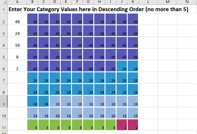
The formula checks the position number of the cell generated by the base formula and sees if it is less than or equal to the number of values in each category in column A. It then returns the value of the category in each cell.
Because I wanted to put symbols in the cell like these examples.

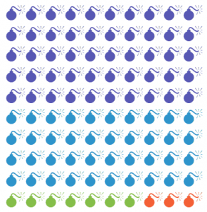
I took that monster formula and made it into a named formula.
This made building the conditional formatting rules much easier to do(simply because the conditional formatting dialog is so cramped).
Lastly, I built a series of conditional formatting rules to change the background colour of the cell based on the value returned by the formula. For the waffles using symbols, the rule formats the colour of the font, instead of the background.
A couple of additional pointers
- To create a perfect grid, switch the view in Excel to Page Layout View. Page Layout View uses the same measurement scale for both row height and column width. Set your measurements here.
- For the symbol waffles, use the File> Options>Advanced> Display Options for this worksheet and turn off the display of gridlines. That way when you copy the waffle, the gridlines will be invisible.
This post is originally from 2018. If you want help with the newest and classic features in Excel & PowerPoint drop me a line at catharine@mytechgenie.ca

