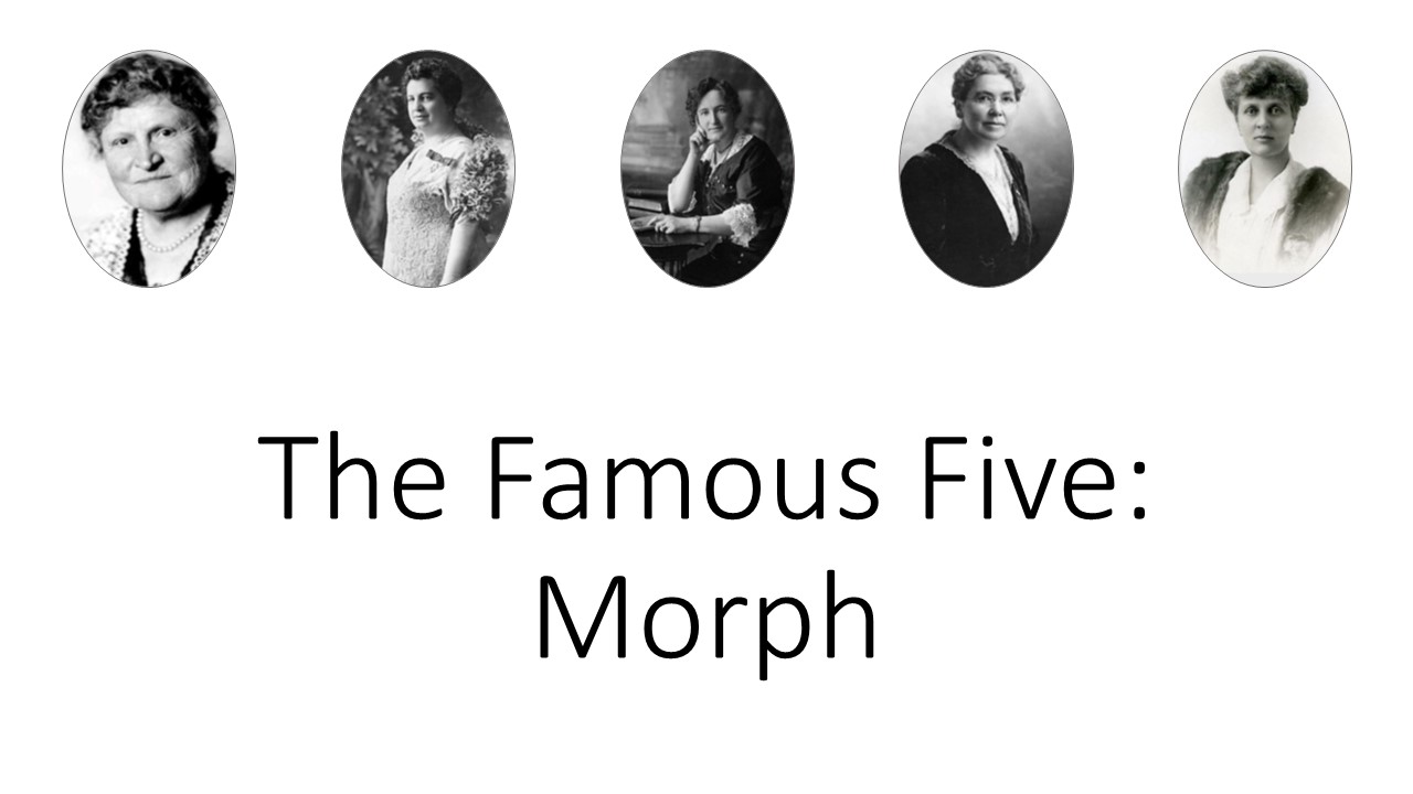
Excel – Total at the Top

It’s that time of year again. Tax time. Now that I’ve made you sad, lets check out a formula which is very useful when adding up long columns of numbers (deductions anyone?)

When you have long columns of numbers of irregular length, it is often easier to have the totals display at the TOP of the page. That way, you don’t have to scroll all over the place to find them. The other advantage of this formula is that you can use it to keep an eye on your total as it accumulates, since you don’t have to know how many rows long the column will be.

The formula here is =SUM(OFFSET(A1,1,0,COUNT($A:$A),1))

Where the OFFSET & COUNT functions are used to create the range that will be summed.

The syntax for OFFSET
OFFSET(reference, rows, cols, [height], [width])
OFFSET(A1,1,0,COUNT($A:$A),1)

  • A1 is the reference cell,
  • Rows – the range begins 1 row down from A1,
  • Cols – the range begins in the same column 0,
  • Height – the number of rows to be included are counted using the COUNT function, COUNT($A:$A) counts the cells in Column A with numbers in them
  • Width – is set to 1 column (column A) wide

I have to say there is something very satisfying about seeing that total increase as each number is entered in the column.

featured image by
Antoine Dautry


This post is originally from 2018 If you want help with the newest and classic features in Excel drop me a line at catharine@mytechgenie.ca

PowerPoint – Organizing your colours

I find it useful when creating a presentation that has a custom colour palette to create a custom layout like the one below:

Colour Palette Assignment Slide Layout – accessible via Master view, or by selecting the layout

You’ll note that the RGB values for the colours are listed, and this is because prior to PowerPoint 2013, the eyedropper tool was not available. I also find it tremendously helpful to note what I use each colour for, so that when I open this file in a couple of years from now there will be a little less detective work.


This post is originally from 2018 If you want help with the newest and classic features in PowerPoint drop me a line at catharine@mytechgenie.ca

PowerPoint: Like toppings on pizza

You may never have looked at Outline View in PowerPoint. But, if you have presentation that has text you should check it out. Working in Outline View is not only the fastest way to build the outline, it creates a more robust and easily edited presentation as well.

By default, when you add text in Outline view, the text is placed in a text placeholder. Placeholder text is easier to edit than text in text boxes.

Here is a little experiment you can do.

Start by adding some text in Outline view. The default Layout “Title and Content” is used.

Looking at a slide in Outline View. The text appears in both the Outline View and the slide.


Here is what the slide looks like in Slides View, again the text is the same in the Slides View panel and in the slide itself.

The Slides View panel

Now try changing the layout to one without a content placeholder. The text remains in Outline View and on the placeholder in the slide. Then, move the text placeholder around and resize it.

Now, change the layout back to “Title and Content” and you’ll find the placeholder snaps back to its original position and size. If you tried recolouring the text, press the Reset button (just underneath the Layout button) and it too will revert to the default appearance set by the placeholder.

Now, compare this with the behaviour of text in text boxes.

This text is in a text box. Note that it does not appear in Outline view.

This text is not connected with the placeholder on the slide. It is “floating” on top of the slide “like toppings on a pizza” in the poetic words of one of my former coworkers.

This lack of connection can make it harder to manage in the long run.

Text box text in slide with placeholders. Text box text in slide with placeholders.

Note what happens when I change the layout to “Title and Content“. The text box is actually floating underneath the placeholder. What a pain for editing! Resetting the slide has no impact on text in text boxes. Also, you’ll notice that the text is not visible in Outline View, so none of those tools are available for editing either.

Does that mean that I never use text boxes?

Of course not, I use text boxes when I want to create text that will remain independent of the general formatting rules for the presentation. But since consistency in formatting is a sign of a professional presentation, I use text boxes sparingly.


This post is originally from 2016. If you want help with the newest and classic features in PowerPoint drop me a line at catharine@mytechgenie.ca

Excel – Find the Last Row and the AGGREGATE Function

Here is a common scenario for me. I like to apply alternate line formatting on spreadsheets, especially wide spreadsheets. It makes it easier to follow the correct row across the spreadsheet. Here a blue fill is applied to alternate lines.

Alternate line formatting

But in this spreadsheet, I wanted to do something a little different. I wanted the alternate line formatting only be applied once the date is entered.

The Alternate Line formatting is not applied until a date is entered.

This means I need to find the last row in the date column. Now previously I’ve used a COUNTIF formula, to count the number of rows with data. Then subtract any blank rows at the top of the spreadsheet. The drawback of this formula, is that editing the spreadsheet later often means the COUNTIF is no longer correct. Gaps in the data also cause problems.

Enter the AGGREGATE Function

The AGGREGATE function was introduced in Excel 2010. Bill Jelen called it “SUBTOTAL on steroids”. It offers 8 more functions than SUBTOTAL and the ability to ignore hidden rows and error values. You can use it either in a Reference or Array form. Here is a link to the MS Support article. One of the new functions offered is LARGE.

So this formula uses
=AGGREGATE(14,6,ROW(A:A)/(NOT(ISBLANK(A:A))),1)
14 – refers to the LARGE function
6 – tells it to ignore error values
ROW(A:A)/(NOT(ISBLANK(A:A))) creates an array of the results of each row number in column A divided by whether the NOT(ISBLANK) portion of the formula returns a TRUE or FALSE answer. TRUE is evaluated as 1 and FALSE as 0. As division by zero creates an error, any blank cells are ignored.
1 – indicates that the LARGE function will return the largest number from the array. Hence, the last row.

The Aggregate function finds the last row
The formula correctly finds the last row, in spite of gaps in the data.

And things came to a grinding halt…

At this point, I did what I normally do and made my AGGREGATE formula into a Named Formula. I typically find this is to be a tidier way of working. When I did this; Excel froze. Repeatedly. Whenever, I did anything that caused a recalculation. Like clicking on a formula to examine it. And if I persisted and used the named formula in the Conditional Formatting formula … things … just … slowed … down … more.

But interestingly, the performance of the spreadsheet doesn’t appear to be affected when the formula is placed in a cell. I was working in Office 2016. I’ll test it later in Office 365, and report back if I get different results. I actually caused the same freezing problem by using the Evaluate Formula button. Excel slows right down as it creates the array of every cell in column A divided by NOT(ISBLANK). Somehow, however, when the formula is in a cell – Excel manages to handle the calculation much more efficiently. I even checked by making the reference to the formula into a named range. No problems. So, if you are planning to use the AGGREGATE function in this way, you’ll need to actually place it somewhere in the spreadsheet. Oh, and you will need to make that cell into a Named Range or else the Conditional Formatting Formula will not work (that was kinda unexpected).

The Conditional Formatting Formula

The formula to produce this conditional formatting is:

=AND(ROW()<=Last_Row,MOD(ROW(),2)=1)
Last_Row refers to cell $B$2
This checks to see if the current row number is less than or equal to the value in the Last_Row Named Range AND if it is an odd numbered row, if so a blue fill is applied.


This post is originally from 2019. If you want help with the newest and classic features in Excel drop me a line at catharine@mytechgenie.ca

A Spreadsheet is Creative (Part 5)

While the content of the spreadsheet is complete, the design isn’t finished yet. I think the best spreadsheets are “scannable”, in other words the reader can scan the sheet and get a sense of the pattern of information, before they even read it. I want the reader to be able to see at a glance whether it is a Facebook or Twitter Post, and to have a sense of the time of day the post will occur. Colour is going to make this happen. Since I have no intention of manually formatting the calendar, Conditional Formatting will make this happen.

A weekly calendar view of the same information.

I am a big fan of conditional formatting, but the working dialog where formulas are added leaves a lot to be desired. So when I base a conditional format on a formula, I will typically build the formula in the spreadsheet so it can be tested and then copy it out of the formula bar and paste it into the working dialog. In this spreadsheet I have 12 (TWELVE) conditional formats, so I ended up pasting the formulas into notepad, so that I could jump back and forth without having to close/reopen the dialog box repeatedly.
I thought quite a bit about how I wanted different times to be represented by colour. I eventually decided on 6 different time “zones”.

  • 10 pm to 7 am
  • 7 am to 9 am
  • 9 am to 12 pm
  • 12 pm to 3 pm
  • 3 pm to 6 pm
  • 6 pm to 10 pm

I needed to find the excel versions of those, so I went to an empty spreadsheet, typed in the time and removed the time format. This is what I found:

Excel time format, converted to the underlying number value

Here are the series of formulas I used for conditional formatting, the first in each group is the default which will format the 10 pm to 7 am time entries.

=(C5=”FB”)
=AND(C5=”FB”,B5>=0.292,B5<0.375)
=AND(C5=”FB”,B5>=0.375,B5<0.5)
=AND(C5=”FB”,B5>=0.5,B5<0.625)
=AND(C5=”FB”,B5>=0.625,B5<0.75)
=AND(C5=”FB”,B5>=0.75,B5<0.917)

=(C5=”TW”)
=AND(C5=”TW”,B5>=0.292,B5<0.375)
=AND(C5=”TW”,B5>=0.375,B5<0.5)
=AND(C5=”TW”,B5>=0.5,B5<0.625)
=AND(C5=”TW”,B5>=0.625,B5<0.75)
=AND(C5=”TW”,B5>=0.75,B5<0.917)

I chose two different colours, based on the http://colorbrewer2.org/ color blind safe palettes and then picked increasingly darker shades of each colour.
And that wraps up this spreadsheet build! I hope you found this look at my process interesting, and I hope that you find building your spreadsheets as creatively satisfying as I do.


I offer Excel template design services and training. Feel free to send me an email – catharine@mytechgenie.ca
Headline image by Kelly Sikkema

A Spreadsheet is Creative (Part 3)

Now, I need to start to pull the post type, time of post and post content from the Content sheet. Starting with the post type (which resides in Column C), the following INDEX function in cell B6 will do the trick:
=INDEX(Content!$C$1:$C$1187,B5,1)
This index formula uses the value from B5 to find the entry in row 530. And yes, at this point that is only the first entry for the day.

Index and If function results

Now, I’ll use an IF statement to build the formulas you see in column C6:
=IF(ROW()<6+C$5,”yes”,”stop”)
At this stage in the process I usually use the IF statement to display a label. “Yes”, means there is matching data in the source sheet. “Stop” means there is no longer matching data. The test in column F shows the formula is working.
Now I’ve proven that the each formula works in turn, I can combine them into a larger “mega” formula. Don’t forget that when building these larger formulas you can; expand the formula bar and use Alt+Enter to force the formula to wrap for easier reading.
Like this:
=IF(ROW()<5+(COUNTIFS(Content!$E:$E,”>=”&B$4,Content!$E:$E,”<“&B$4+1)),
INDEX(Content!$C:$C,(MATCH(B$4,Content!$E:$E,0)),1),”stop”)
You’ll notice that I’ve also stopped referring to a specific range in column E/C and instead reference the entire column. It doesn’t make any difference to the result of this formula and makes it a bit simpler to read. Also the Row adjustment number changes from 6 to 5 as I play with the layout of the spreadsheet. Changing the layout includes reordering the data, so that the time of the post comes first and adding a column that shows the path to any images used in the post.

Here’s a shot of the results of that formula:

The formula is expanded to more columns Now I’m capturing more columns of data

You’ve undoubtedly spotted that only the first entry is being captured and repeated. I’ll adjust the formula to correct that problem in my next post.


I offer Excel template design services and training. Feel free to send me an email.

Headline Image from William Iven

A Spreadsheet is Creative – Part 1

Creating a spreadsheet is a creative act. The choices made about data, formulas, layout and colour all contribute to communicating clearly. Communicating clearly and well is, in my book a creative process.

So, I thought I’d walk through my process in designing a spreadsheet to take information from what is essentially a database layout:

This database view works fine for an Excel Nerd like me.

Into this view, a classic calendar view of the same information:

A weekly calendar view of the same information.

I’m planning to use the calendar view to share a social media posting schedule, as the people I’m sharing with aren’t Excel savvy (and why should they be?). I create the posting schedule in Excel, because I can easily save it in .csv format and upload it to Google Calendar. However, sharing the Google Calendar has drawbacks too, and it is simpler to print out a weekly calendar showing the planned posts.
When I began this process, I had some things sketched out in my mind. I wanted to enter a date and see the week around it. I always want to see the posts for the date in the context of the posts for the days around it. I also want a consistent layout of days – Sunday to Monday. Having the starting day of the week change each time would make it harder for my viewers.
That means I’m going to need to dynamically generate the dates based on the day of the week of my starting date. You can see my first pass below:

Dynamically generating the date based on the day of the week

I labelled cell A1 WeekStart, this will help me remember the purpose of the contents of cell A1.
I’ve labelled the days of the week, and above them in row 2, given each day a number 1-7. The day numbers relate to the way the WEEKDAY function works. I’ll be using the mode where the week starts numbering 1 on Sunday. Later I’ll hide that row, but for now having it visible is helpful.
You can see that I’m stepping out the formula in rows 4 – 6. When I’m designing a spreadsheet, I’ll often step formulas out like this. It helps me avoid errors and makes each step clear. Later I’ll consolidate the steps.
In row 4, I’m calculating the following:
=(WEEKDAY(WeekStart,1))-B$2.
You can think of it as a way to calculate the number of days (+/-) from my start date. By the way, I chose to start with May 1, because it was on a Wednesday. That made sure I could test my formulas well, a Saturday or Sunday starting day would make testing harder.
Once I know I can count backwards and forwards from my starting date, I use the following formula:
=WeekStart-((WEEKDAY(WeekStart,1))-B$2)
The WEEKDAY function calculates the day number of the week. Here, it returns the number 4(Wednesday).
From the number 4 I subtract the value in row 2. This gives me the number of days to subtract from the WeekStart value. You can see the results in rows 5 and 6. Row 5 is simply the unformatted date value, since sometime I find visualizing the pure number easier.

This turned out to be a 5 part series! I hope you’ll find the next 4 parts interesting.

I’ll continue with the design process in my next post.


I offer Excel template design services and training. Feel free to send me an email – catharine@mytechgenie.ca

Headline Photo by Estée Janssens on Unsplash

The Word Navigation Pane

The Navigation Pane

Among the many reasons I love Word Styles, is how it makes the Navigation Pane more powerful and easier to use.

Find Navigation Pane on the View Ribbon

Turn on the Navigation Pane by going to the View Tab, Show Group and checking the Navigation Pane check box.

Unformatted text on the page and in Navigation Pane

At this point, if your text is unformatted, the Navigation Pane will not look that useful. But, watch what happens when I add styles to the unformatted text.

Text Formatted with Styles appears both on the page and in the Navigation Page

Now the text appears in the Navigation Page in the same style hierarchy used in the document. Now I can use the Navigation Page to quickly move around the document by clicking on the text I want to jump to.

Text can be collapsed and expanded

If there is a lot of text, it can be collapsed and expanded using the triangle buttons.
The Navigation Pane can be used for more than navigation, it can also be used to reorder/reorganize text in the document. For example, perhaps I wish to move the section on the “The Adventures of Pinocchio” after “Aladdin”. I can do this easily by clicking on that heading in the Navigation Pane and dragging it below the heading I want it to follow.

Results of using the Navigation Pane to reorder my document

Not only is that heading moved but all the subtext beneath it is moved as well. Fast and easy document reorganization!


I offer Word template design services and training. Feel free to send me an email.
Featured image from
oxana v

One File to Many – MS Word

A few weeks ago the following request came to me: “I have also been told that there is a way to change and update several … in a bulk fashion, that would speed up the process when customizing many documents for a specific job.” Of course, I immediately started thinking about a process that would allow one to smoothly update a group of standard documents. For example; every time a new customer is being set up.

I reached for the INCLUDETEXT field in Word. In contrast to inserting a file (which takes the entire contents of a file), the INCLUDETEXT field allows you to specify text within a file, when that text has been identified by a bookmark.

The Plan

Set up a “CustomerInfo” source document. Then in my standard documents (target documents), I’d use the INCLUDETEXT field to link to the relevant pieces of information stored in the source document. Updating would be a breeze, simply change the information in the source and the next time the fields are updated in the target document all the correct information will appear. In this process, the Customer Information source document would:

  1. Always have the same file name
  2. Be stored in the same folder as the rest of the customer files. If this is not the case, then the field code in the target document will need to be adapted from my example.

The Source Document

Setting up the source document is pretty straightforward – I’d make a form detailing the information to be collected. However, bookmarks are too easy to delete when adding or updating information. I’d use content controls nested inside the bookmarks. This also takes advantage of tabbing from one control to another, making it faster to input and edit information. The controls can be grouped or placed in a table. But don’t use the Locking options when creating the control. Locking a control prevents the target document from updating.

The Target Document

I’d place the following field in the target document
{INCLUDETEXT "{FILENAME \P}\\..\\source document filename" bookmark}
Replacing the source document filename with the Customer Information filename (including the docx extension) and the bookmark with the name of the bookmark from the source document.
The {FILENAME \P}\\..\\ portion of the field extracts the path & filename of the current file and clips off the filename (using \\..\\), which allows you to substitute the source document filename. Hat tip to MS Word MVP Paul Edstein for this clever solution.

Updating

The INCLUDETEXT field is classified as a “warm” field in Word. This means it does not update automatically, but requires user intervention. The user needs to select the field and press the F9 function key to update. If multiple fields are used in the same document, use Ctrl + A to select the entire document, then press F9 to update all fields.
There are macros to update all the fields as well, but the keyboard commands are just as straightforward. Depending on the workflow, I might write a macro to loop through all the documents in a folder and force updating.

I offer Word template design services and training. Feel free to send me an email.

Duotone Photo Technique

Duotone Photos

I’ve been showing you how to use PowerPoint to quickly create stencil and lace effects. Now, let’s look at creating duotone photos. In addition to making a photo look very modern, duotone is a useful technique for using less than stellar photos.

Cat in the Kitchen

While the cat might be photogenic, the background is not. I want to move from the photo above to the duotone below, which is suitable for adding a quote.

So true

The first step is to crop the picture as closely as possible.

Just the handsome face here – no clutter

But unfortunately, once enlarged you see the photo is a little blurry. This won’t be a problem going forward and it shows how this technique can cope with less than perfect photos.

Going to Picture Corrections:
Brightness was set to 65%
Contrast to 100%

Picture Color: Saturation was set to zero.

The Adjusted Photo

There is a bit of guesswork here, as I had to bring up Brightness enough to wash out the dark corner of the chair the cat is on, yet leave as much detail as possible. You’ll note that this brings out a lot of light spots on the pupils as well.

Why not just Recolor the picture to Black and White? In this case, I felt that recoloring removed too much detail from the photo. In the case of a different photo, recoloring might be the quickest and easiest method. I’d definitely try it first and see if I liked the results.

I’ve drawn a rectangle and filled it with a bright colour for contrast, this has been placed under the photo.

Now I can make the white portion of the photo transparent, by selecting Picture Tools>Format>Color>Set Transparent Color and clicking on a white portion of the picture.

The black portion of the photo remains.

What’s also hard to see in the above picture is that the photo has a lot of small grey artifacts in the borders of the fur. This is exactly what we added in when making the lace picture earlier, but here it is unwanted. An additional step is required for this photo (again for some photos it might be unnecessary).

But before I do that – I’m going to use the Ink command and touch up the pupils to remove some of the glints. Ink is only available in Office 365.

Showing Glint repair using ink tool.

After filling in the glints on the pupils, I grouped the ink layer with the photo. Then I copied and pasted the photo (and ink layer) as a picture. PowerPoint remembers all the photo editing done to a picture (which is why the Reset command works) and applies those steps cumulatively. I want to start fresh and apply the Recolor command to strip out the grey artifacts without losing a lot of detail. After recoloring the photo to 25% Black and White I set the White color to transparent

The same photo, but now with a crisper look

Again, I grouped the photo with bright background rectangle, pasted it as a picture and this time set the black portion as transparent. This is similar to the photo stencil.

Photo with transparent cat

In the final step, set a gradient fill in your chosen colour scheme to colour the duotone.

Setting the background of the slide to colour the duotone

The main elements of this technique are applicable to a number of photo effects. Try them out and see what you get!


This post is originally from 2018 If you want help with the newest and classic features in PowerPoint drop me a line at catharine@mytechgenie.ca