Fine-Tuning PowerPoint’s Morph Function

Using Morph

It’s October 18 – Persons Day. On this day in 1929, the Judicial Committee of the Privy Council in Great Britain made the decision to include women under the legal definition of persons in Canada. This landmark was thanks to the efforts of the Famous Five, a group of Albertan suffragettes whose names were Henrietta Muir Edwards, Emily Murphy, Nellie McClung, Louise McKinney, and Irene Parlby.

I figured this would be a great opportunity to test out PowerPoint 2019’s morph function in order to create a presentation honouring the Famous Five. I started with an image of these women in elliptical frames, all taken at roughly the same distance. I then made four duplicates, and used PowerPoint’s Remove Background feature so that I had one image of each individual woman. I lined these up at the top of the title slide, and then duplicated the slide four times. I used the morph function to blow up each woman’s photo in turn, with each previous photo receding back up to the top row once her individual profile was clicked through.

Morph isn’t Perfect

My plan, however, wasn’t foolproof. I noticed that in several of the transitions, the large image and the small one that replaced it would not glide towards each other’s positions. Instead, invisible versions of the original uncropped image would glide around within the crop frame, each image refocusing on its new subject independently.

Fixing the Problem

To solve this, we took five oval shapes and sized them to fit the women’s frames as closely as possible. We then grouped each image with its oval. Now, instead of sliding around the uncropped image, the transition applied to the shape, inflating it and shrinking it as we had hoped.

This, though, allowed us to discover a new problem: on several of the transitions, the image coming to the forefront would abruptly jump through the receding image; clearly, the z-order (position in the imaginary stack of all items on the slide) was not consistent between slides. Simply picking a consistent order and applying it to all slides solved this, but it left us with one more thing to think about.

When issuing forth from the top row, or rejoining it, some of the images would glide just underneath the edges of adjacent images on their way to their final position. I felt that this did not make aesthetic sense; shouldn’t the bigger, “closer” image glide in front of the smaller ones? The thing was, though, that tweaking the z-order to avoid this inevitably led back to the other problem of images jumping through one another.  We solved this by duplicating the problematic images and aligning the duplicate directly overtop of the original; we then animated the duplicate to appear after the last morph transition, with the original disappearing at the same time. This resulted, finally, in a seamless transition.

Shortcuts and Learning

I had a couple of requests for OneNote support this month and decided to take a look at the Office 365 version. Its been a few versions since I used OneNote and I wanted to refresh my understanding of what the software capabilities are. One of the things I looked at (in addition to building custom templates) were the shortcuts in the program.

I would never try to learn software from shortcuts, but I do find it useful to see what shortcuts the developers have built-in to a product. It shows what features they believe are most useful and popular.  When I spot a cluster of shortcuts like these:

Ctrl + 0  Remove all selected note tags
Ctrl + 1   Apply, select or clear the to do tag toggles through all options
Ctrl + 2   Toggles the important tag
Ctrl + 3   Toggles the question tag
Ctrl + 4   Toggles the remember for later tag
Ctrl + 5   Toggles the definition tag
Ctrl + 6   Toggles the highlight tag
Ctrl + 7   Toggles the contact tag
Ctrl + 8   Toggles the address tag
Ctrl + 9   Toggles the phone number tag

Then I can be sure that Tags are an important feature in the product.
When shortcuts have been assigned an easy to access and remember combination like Ctrl or Ctrl Shift indicates the priority level of the feature:

Ctrl Shift + 0   Delete the selected Outlook task
Ctrl Shift + 1    Create a today Outlook task from the selected note
Ctrl Shift + 2   Create a tomorrow Outlook task from the selected note
Ctrl Shift + 3   Create a this week Outlook task from the selected note
Ctrl Shift + 4   Create a next week Outlook task from the selected note
Ctrl Shift + 5   Create a no date Outlook task from the selected note
Ctrl Shift + 9   Mark the selected outlook task as complete
Ctrl Shift + E   Send the selected pages in an email message
Ctrl Shift + K   Open the selected Outlook task

Then I know the developers expect these functions to be frequently used.

Learning new software can feel overwhelming when you have a long To Do list. Spotting shortcut key clusters and priority patterns can help you to prioritize which features to learn first.

Oops! I closed that tab! (in Windows 10)

You’re working on a research project, and you’ve dug through the bowels of the internet to find some information that is relevant to your question. After a brief interlude of looking up which artist sang the song you have stuck in your head in a new tab, your caffeine-saturated finger muscles accidentally press the close button/Ctrl + W one too many times. Oh no! We’ve all been there, but not all of us know what to do about it. Until now.

Press Ctrl + Shift + T to reopen the tab you’ve just closed, and the tab you closed before that, and so on. What’s more, if your computer updated overnight and closed your browser, you can use this same trick after you open your browser back up to recall all the tabs that you lost. This trick works in every browser on Windows 10.

Windows 10 MAGNIFY!

Another day at work, and your boss is checking in to see what you’ve accomplished. Of the several windows you have open, both for the project and for reference, one has very small text, and another has a font colour that doesn’t stand out against the background. How can you show your boss your progress without them having to squint 6 inches away from your screen? Or perhaps you’re presenting an Excel spreadsheet to a huge room. How can you make sure the people at the back can see the values in the cells?

Windows 10’s magnifier shortcut is your easy accommodation for this problem. By pressing Windows Logo Key + = (equals), you can zoom your screen in on wherever your cursor sits. This shortcut comes in three versions. In Full Screen Version (Ctrl + Alt + F), the entire screen zooms in on your cursor. In Lens Version ( Ctrl + Alt + L), a small window showing the magnified area appears. In Docked Version (Ctrl + Alt + D), the magnified area is displayed in a wide panel that appears at the top of the screen. These versions can be cycled between using Ctrl + Alt + M. In all three versions, the area magnified changes depending on where you move your mouse, and each version is also accompanied by a miniature window which allows you to:

  • Change the degree of magnification
  • Access a text-to-speech feature
  • Change the speed and accent of the text-to-speech feature*

Exit the magnifier by pressing Windows Logo Key + Esc.

Windows 10 Emojis: A Shortcut

Imagine that you’re a CSIS agent, and you’ve been asked to write up a report regarding the text messages exchanged between two suspects in a terror plot. Straightforward enough – unless the suspects use emojis. What is your senior agent going to think if your report states that one suspect used the “exploding head” emoji? Without a way to show the emojis themselves in high resolution, confusion might ensue.

Of course, you could have plenty of mundane reasons to want emojis in your documents as well. Perhaps you want your emails in Outlook to seem more approachable, or maybe you want to construct a simulated text conversation on a PowerPoint slide. Fortunately, Windows 10 has a solution: a searchable emoji keyboard. This tool can be called upon in almost any Windows 10 app by pressing the  Windows Logo Key + . (period). The dialogue box that appears is the same in any app that you open it in, and has all the same emoji options that you have on your phone, as well as pre-made “kaomojis” [(づ ̄3 ̄)づ╭❤~, (❁´◡`❁), etc.]. You can keep typing in the same spot in the document to search for a specific emoji, or you can click on the dialogue box’s various category tabs to view related options.

Excel – Total at the Top

It’s that time of year again. Tax time. Now that I’ve made you sad, lets check out a formula which is very useful when adding up long columns of numbers (deductions anyone?)

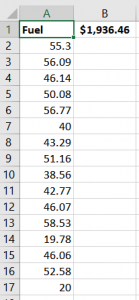
When you have long columns of numbers of irregular length, it is often easier to have the totals display at the TOP of the page. That way, you don’t have to scroll all over the place to find them. The other advantage of this formula is that you can use it to keep an eye on your total as it accumulates, since you don’t have to know how many rows long the column will be.

The formula here is =SUM(OFFSET(A1,1,0,COUNT($A:$A),1))

Where the OFFSET & COUNT functions are used to create the range that will be summed.

The syntax for OFFSET
OFFSET(reference, rows, cols, [height], [width])
OFFSET(A1,1,0,COUNT($A:$A),1)

  • A1 is the reference cell,
  • Rows – the range begins 1 row down from A1,
  • Cols – the range begins in the same column 0,
  • Height – the number of rows to be included are counted using the COUNT function, COUNT($A:$A) counts the cells in Column A with numbers in them
  • Width – is set to 1 column (column A) wide

I have to say there is something very satisfying about seeing that total increase as each number is entered in the column.

featured image by
Antoine Dautry


This post is originally from 2018 If you want help with the newest and classic features in Excel drop me a line at catharine@mytechgenie.ca

PowerPoint – Organizing your colours

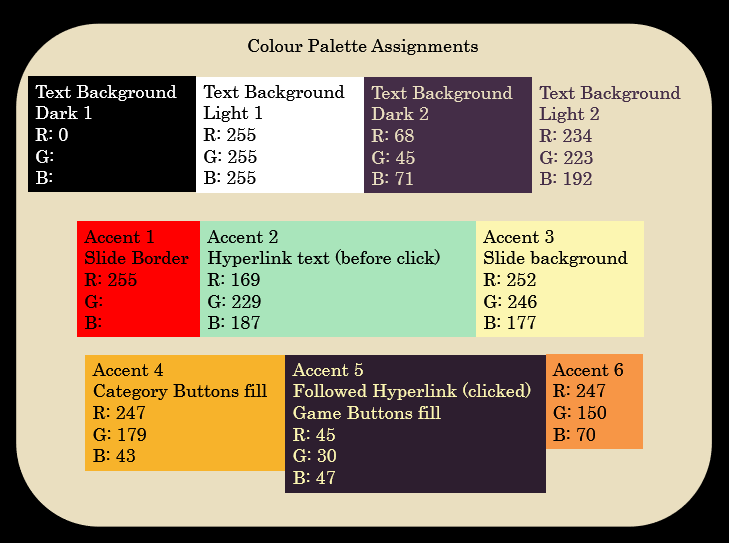
I find it useful when creating a presentation that has a custom colour palette to create a custom layout like the one below:

Colour Palette Assignment Slide Layout – accessible via Master view, or by selecting the layout

You’ll note that the RGB values for the colours are listed, and this is because prior to PowerPoint 2013, the eyedropper tool was not available. I also find it tremendously helpful to note what I use each colour for, so that when I open this file in a couple of years from now there will be a little less detective work.


This post is originally from 2018 If you want help with the newest and classic features in PowerPoint drop me a line at catharine@mytechgenie.ca

January 2023 Teaching Schedule

 Foxit: PDF Editor Medicine Hat College Continuing Studies
January 18-19, 2023

When Adobe moved to a subscription model for all its products, other businesses moved in to offer their stand alone software. One of those products is Foxit’s PDF Editor. What is PDF Editor Software? With a PDF Editor you can edit the contents of a PDF; changing text and images, reordering and deleting pages, create forms, add and update headers and footers, add and update watermarks, assemble new PDF documents from multiple sources, and redact documents. There is a lot you can do with a PDF editor, so much that it required a TWO day course to cover it all.

Microsoft Excel: Formulas and Functions Medicine Hat College Continuing Studies
January 27, 2023

Need to feel more confident about building formulas and using common Excel functions? Try this one day course. Among other topics, you’ll learn about absolute and relative references.

This course will also run in June.


PowerPoint: Like toppings on pizza

You may never have looked at Outline View in PowerPoint. But, if you have presentation that has text you should check it out. Working in Outline View is not only the fastest way to build the outline, it creates a more robust and easily edited presentation as well.

By default, when you add text in Outline view, the text is placed in a text placeholder. Placeholder text is easier to edit than text in text boxes.

Here is a little experiment you can do.

Start by adding some text in Outline view. The default Layout “Title and Content” is used.

Looking at a slide in Outline View. The text appears in both the Outline View and the slide.


Here is what the slide looks like in Slides View, again the text is the same in the Slides View panel and in the slide itself.

The Slides View panel

Now try changing the layout to one without a content placeholder. The text remains in Outline View and on the placeholder in the slide. Then, move the text placeholder around and resize it.

Now, change the layout back to “Title and Content” and you’ll find the placeholder snaps back to its original position and size. If you tried recolouring the text, press the Reset button (just underneath the Layout button) and it too will revert to the default appearance set by the placeholder.

Now, compare this with the behaviour of text in text boxes.

This text is in a text box. Note that it does not appear in Outline view.

This text is not connected with the placeholder on the slide. It is “floating” on top of the slide “like toppings on a pizza” in the poetic words of one of my former coworkers.

This lack of connection can make it harder to manage in the long run.

Text box text in slide with placeholders. Text box text in slide with placeholders.

Note what happens when I change the layout to “Title and Content“. The text box is actually floating underneath the placeholder. What a pain for editing! Resetting the slide has no impact on text in text boxes. Also, you’ll notice that the text is not visible in Outline View, so none of those tools are available for editing either.

Does that mean that I never use text boxes?

Of course not, I use text boxes when I want to create text that will remain independent of the general formatting rules for the presentation. But since consistency in formatting is a sign of a professional presentation, I use text boxes sparingly.


This post is originally from 2016. If you want help with the newest and classic features in PowerPoint drop me a line at catharine@mytechgenie.ca

Excel – Find the Last Row and the AGGREGATE Function

Here is a common scenario for me. I like to apply alternate line formatting on spreadsheets, especially wide spreadsheets. It makes it easier to follow the correct row across the spreadsheet. Here a blue fill is applied to alternate lines.

Alternate line formatting

But in this spreadsheet, I wanted to do something a little different. I wanted the alternate line formatting only be applied once the date is entered.

The Alternate Line formatting is not applied until a date is entered.

This means I need to find the last row in the date column. Now previously I’ve used a COUNTIF formula, to count the number of rows with data. Then subtract any blank rows at the top of the spreadsheet. The drawback of this formula, is that editing the spreadsheet later often means the COUNTIF is no longer correct. Gaps in the data also cause problems.

Enter the AGGREGATE Function

The AGGREGATE function was introduced in Excel 2010. Bill Jelen called it “SUBTOTAL on steroids”. It offers 8 more functions than SUBTOTAL and the ability to ignore hidden rows and error values. You can use it either in a Reference or Array form. Here is a link to the MS Support article. One of the new functions offered is LARGE.

So this formula uses
=AGGREGATE(14,6,ROW(A:A)/(NOT(ISBLANK(A:A))),1)
14 – refers to the LARGE function
6 – tells it to ignore error values
ROW(A:A)/(NOT(ISBLANK(A:A))) creates an array of the results of each row number in column A divided by whether the NOT(ISBLANK) portion of the formula returns a TRUE or FALSE answer. TRUE is evaluated as 1 and FALSE as 0. As division by zero creates an error, any blank cells are ignored.
1 – indicates that the LARGE function will return the largest number from the array. Hence, the last row.

The Aggregate function finds the last row
The formula correctly finds the last row, in spite of gaps in the data.

And things came to a grinding halt…

At this point, I did what I normally do and made my AGGREGATE formula into a Named Formula. I typically find this is to be a tidier way of working. When I did this; Excel froze. Repeatedly. Whenever, I did anything that caused a recalculation. Like clicking on a formula to examine it. And if I persisted and used the named formula in the Conditional Formatting formula … things … just … slowed … down … more.

But interestingly, the performance of the spreadsheet doesn’t appear to be affected when the formula is placed in a cell. I was working in Office 2016. I’ll test it later in Office 365, and report back if I get different results. I actually caused the same freezing problem by using the Evaluate Formula button. Excel slows right down as it creates the array of every cell in column A divided by NOT(ISBLANK). Somehow, however, when the formula is in a cell – Excel manages to handle the calculation much more efficiently. I even checked by making the reference to the formula into a named range. No problems. So, if you are planning to use the AGGREGATE function in this way, you’ll need to actually place it somewhere in the spreadsheet. Oh, and you will need to make that cell into a Named Range or else the Conditional Formatting Formula will not work (that was kinda unexpected).

The Conditional Formatting Formula

The formula to produce this conditional formatting is:

=AND(ROW()<=Last_Row,MOD(ROW(),2)=1)
Last_Row refers to cell $B$2
This checks to see if the current row number is less than or equal to the value in the Last_Row Named Range AND if it is an odd numbered row, if so a blue fill is applied.


This post is originally from 2019. If you want help with the newest and classic features in Excel drop me a line at catharine@mytechgenie.ca