Shortcuts and Learning

I had a couple of requests for OneNote support this month and decided to take a look at the Office 365 version. Its been a few versions since I used OneNote and I wanted to refresh my understanding of what the software capabilities are. One of the things I looked at (in addition to building custom templates) were the shortcuts in the program.

I would never try to learn software from shortcuts, but I do find it useful to see what shortcuts the developers have built-in to a product. It shows what features they believe are most useful and popular.  When I spot a cluster of shortcuts like these:

Ctrl + 0  Remove all selected note tags
Ctrl + 1   Apply, select or clear the to do tag toggles through all options
Ctrl + 2   Toggles the important tag
Ctrl + 3   Toggles the question tag
Ctrl + 4   Toggles the remember for later tag
Ctrl + 5   Toggles the definition tag
Ctrl + 6   Toggles the highlight tag
Ctrl + 7   Toggles the contact tag
Ctrl + 8   Toggles the address tag
Ctrl + 9   Toggles the phone number tag

Then I can be sure that Tags are an important feature in the product.
When shortcuts have been assigned an easy to access and remember combination like Ctrl or Ctrl Shift indicates the priority level of the feature:

Ctrl Shift + 0   Delete the selected Outlook task
Ctrl Shift + 1    Create a today Outlook task from the selected note
Ctrl Shift + 2   Create a tomorrow Outlook task from the selected note
Ctrl Shift + 3   Create a this week Outlook task from the selected note
Ctrl Shift + 4   Create a next week Outlook task from the selected note
Ctrl Shift + 5   Create a no date Outlook task from the selected note
Ctrl Shift + 9   Mark the selected outlook task as complete
Ctrl Shift + E   Send the selected pages in an email message
Ctrl Shift + K   Open the selected Outlook task

Then I know the developers expect these functions to be frequently used.

Learning new software can feel overwhelming when you have a long To Do list. Spotting shortcut key clusters and priority patterns can help you to prioritize which features to learn first.

The Word Navigation Pane

The Navigation Pane

Among the many reasons I love Word Styles, is how it makes the Navigation Pane more powerful and easier to use.

Find Navigation Pane on the View Ribbon

Turn on the Navigation Pane by going to the View Tab, Show Group and checking the Navigation Pane check box.

Unformatted text on the page and in Navigation Pane

At this point, if your text is unformatted, the Navigation Pane will not look that useful. But, watch what happens when I add styles to the unformatted text.

Text Formatted with Styles appears both on the page and in the Navigation Page

Now the text appears in the Navigation Page in the same style hierarchy used in the document. Now I can use the Navigation Page to quickly move around the document by clicking on the text I want to jump to.

Text can be collapsed and expanded

If there is a lot of text, it can be collapsed and expanded using the triangle buttons.
The Navigation Pane can be used for more than navigation, it can also be used to reorder/reorganize text in the document. For example, perhaps I wish to move the section on the “The Adventures of Pinocchio” after “Aladdin”. I can do this easily by clicking on that heading in the Navigation Pane and dragging it below the heading I want it to follow.

Results of using the Navigation Pane to reorder my document

Not only is that heading moved but all the subtext beneath it is moved as well. Fast and easy document reorganization!


I offer Word template design services and training. Feel free to send me an email.
Featured image from
oxana v

One File to Many – MS Word

A few weeks ago the following request came to me: “I have also been told that there is a way to change and update several … in a bulk fashion, that would speed up the process when customizing many documents for a specific job.” Of course, I immediately started thinking about a process that would allow one to smoothly update a group of standard documents. For example; every time a new customer is being set up.

I reached for the INCLUDETEXT field in Word. In contrast to inserting a file (which takes the entire contents of a file), the INCLUDETEXT field allows you to specify text within a file, when that text has been identified by a bookmark.

The Plan

Set up a “CustomerInfo” source document. Then in my standard documents (target documents), I’d use the INCLUDETEXT field to link to the relevant pieces of information stored in the source document. Updating would be a breeze, simply change the information in the source and the next time the fields are updated in the target document all the correct information will appear. In this process, the Customer Information source document would:

  1. Always have the same file name
  2. Be stored in the same folder as the rest of the customer files. If this is not the case, then the field code in the target document will need to be adapted from my example.

The Source Document

Setting up the source document is pretty straightforward – I’d make a form detailing the information to be collected. However, bookmarks are too easy to delete when adding or updating information. I’d use content controls nested inside the bookmarks. This also takes advantage of tabbing from one control to another, making it faster to input and edit information. The controls can be grouped or placed in a table. But don’t use the Locking options when creating the control. Locking a control prevents the target document from updating.

The Target Document

I’d place the following field in the target document
{INCLUDETEXT "{FILENAME \P}\\..\\source document filename" bookmark}
Replacing the source document filename with the Customer Information filename (including the docx extension) and the bookmark with the name of the bookmark from the source document.
The {FILENAME \P}\\..\\ portion of the field extracts the path & filename of the current file and clips off the filename (using \\..\\), which allows you to substitute the source document filename. Hat tip to MS Word MVP Paul Edstein for this clever solution.

Updating

The INCLUDETEXT field is classified as a “warm” field in Word. This means it does not update automatically, but requires user intervention. The user needs to select the field and press the F9 function key to update. If multiple fields are used in the same document, use Ctrl + A to select the entire document, then press F9 to update all fields.
There are macros to update all the fields as well, but the keyboard commands are just as straightforward. Depending on the workflow, I might write a macro to loop through all the documents in a folder and force updating.

I offer Word template design services and training. Feel free to send me an email.

Excel: Frozen

Businessman with Data

Freezing panes is a basic tool to make a large spreadsheet easier to work with. In my social media spreadsheet I like to freeze the header row into position. Then no matter how far I scroll down the sheet, the columns are labelled.

To turn on frozen panes, select the cell below the row & column you wish to freeze into position. Since I don’t want to freeze any columns, I select cell A2.

Freezing Panes using the Active Cell position" width
Freezing Panes using the Active Cell position” width

Select the View Ribbon, Click on the Freeze Panes button, and choose Freeze Panes (or Freeze Top Row in this scenario).

Freezing Panes Results

Now you can scroll for hundreds of rows, and each column is nicely labelled – no guessing!


This post is originally from 2016. If you want help with the newest and classic features in Excel drop me a line at catharine@mytechgenie.ca

Excel: Select Visible (2)

Man hand and laptop
The Select Visible Cells Only button on the Quick Access Toolbar

The Select Visible Cells Only function is so useful, I like to add it to the Quick Access Toolbar (QAT) in Excel. These instructions are based on Excel 2010, but will be similar in all current versions of Excel.

Quick Access Toolbar Customization

The Quick Access Toolbar starts in the top right corner of the Excel window. The customize button is circled in red. Clicking on that button displays the menu shown below.

Move the QAT under the ribbon

The first change I like to make is to its’ position. I like to move it under the Ribbon, since there will be more room for buttons there. Over time I tend to fill the QAT up with frequently used tools.

After I move the QAT below the ribbon, I go hunting for useful commands to add. Click the More Commands… option and the Customize the Quick Access Toolbar dialog opens up.

Customize the Quick Access Toolbar - Popular Commands
Customize the Quick Access Toolbar – Popular Commands

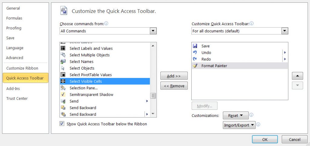
The dialog box defaults to Popular Commands. Try scrolling through this list and find the Format Painter. Press the Add button, to add it to the Quick Access Toolbar. This is a useful tool to have at hand!

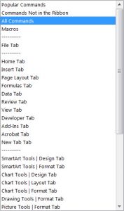
By clicking on the Choose commands from drop-down list, a selection will be displayed.

Drop-down list of source commands.

Select All Commands from this list. Hundreds of Excel commands will display, and this is where it is useful to know the name of the command you are looking for. Scroll until you find Select Visible Cells.

Finding the Select Visible Cells command

Select it, Click on the Add button, and click OK.

Simply select the cells you wish to copy and press the Select Visible Cells button. Paste your information and only what you see will be pasted.


This post is originally from 2016. If you want help with the newest and classic features in Excel drop me a line at catharine@mytechgenie.ca

Excel: Select Visible (1)

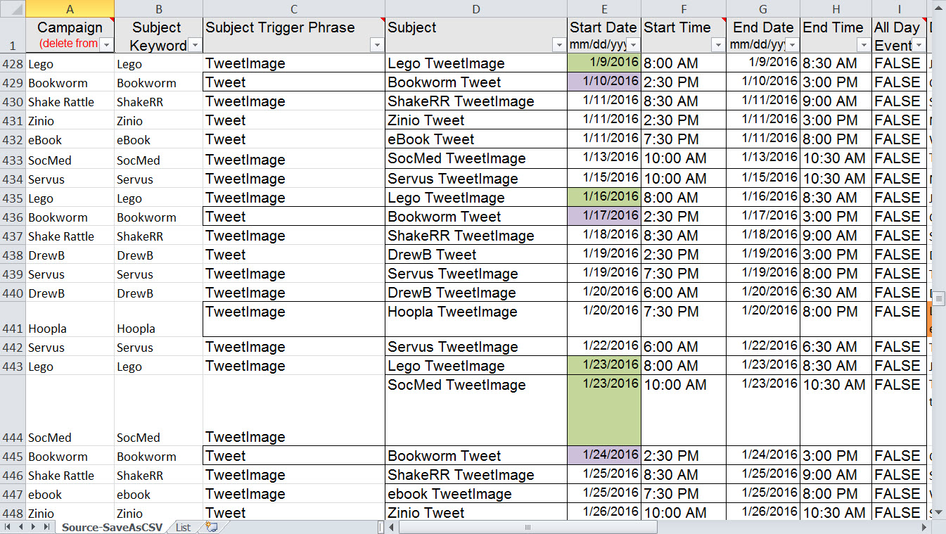
I built my Social Media spreadsheet in an Excel spreadsheet with all the tools I want built in (formulas, conditional formatting and data validation). Ultimately, I will transfer my information into a stripped down spreadsheet in csv (comma separated) format. This is the format that Google Calendars will accept.

When I transfer my posts to this spreadsheet, I don’t want to include any blank rows AND I only want to copy and paste once. How do I perform this little piece of magic? I use the Excel command for selecting visible cells only.

Go To Special Dialog, select Visible cells only

Tucked away in the Go To Special dialog is the option for selecting only the visible cells in a region. This takes what could be multiple copy/paste operations and condenses them into one step.

First filter your data so that blanks do not appear, then press the F5 function key to bring up the Go To dialog box.

Press the Special button to open the Go To Special dialog box, choose Visible cells only and press OK. Now when you copy the selected cells, only the cells you can see are copied.

In my next post I’ll show the method to put this useful button on your Quick Access Toolbar.


This post is originally from 2016. If you want help with the newest and classic features in Excel drop me a line at catharine@mytechgenie.ca

Excel: Filtering in action

Filtering Data
The Filter Button on the Toolbar
Finding the Filtering button

Since Excel 2007, the Filter tool has been on the Home ribbon, under the Sort and Filter drop-down. The Filter tool can be applied to any spreadsheet where every row is a new record. Excels’ guesses about what and how to filter will be more accurate if the data has a header row. Your (human) life will be easier if you give that row a little formatting to make it stand out from the data.

If your data has gaps, select all the data (including the header row) and apply the filter. Once the filter has been applied, little triangles will appear beside each header label.

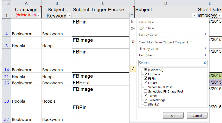
Filtering Drop-Down panel

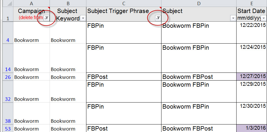
Now you can use each header to filter the data. Click on the filter drop-down and the panel will open as you can see in the picture above. Clear the check boxes beside the entries you don’t want to see. Then click the OK button. You can spot filtered data, because the row headers will be bright blue (and row numbers will be missing as data is filtered out). The columns where filtering is applied will have a filter icon (circled in red in the picture).

Filtering Applied
Filtering Applied

Once the filters are in place, I can filter out blanks or filter blanks in to find openings in our social media schedule. I can quickly look for Posts and Tweets with images, to ensure the image information is present. I can filter down to a single subject. All of these filters make managing my posting schedule MUCH easier.


This post is originally from 2016. If you want help with the newest and classic features in Excel drop me a line at catharine@mytechgenie.ca

Excel: Validate!

DataValidationdropdown

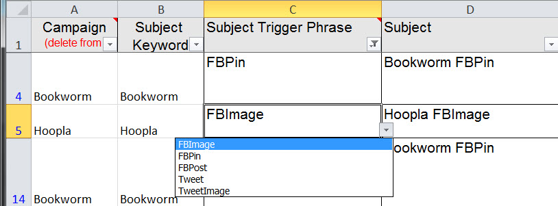
When building my Social Media spreadsheet, I want to enter my subject keywords and trigger keywords consistently. Minor typos can make it difficult to find all the relevant posts and worse; prevent scheduled posts, tweets and pins from being published on time. This is why I find the Data Validation feature in Excel so useful. As you can see in the picture above, once Data Validation is in action, my data entry is restricted to a preset list of options.

Data Validation Ribbon
Find the Data Validation tool on the Data ribbon

Since Excel 2007, the Data Validation tool has been on the Data Ribbon. Simply select the cells you want to apply Data Validation to and press the Data Validation button and select Data Validation. Then the Data Validation Settings dialogue box will appear.

Data Validation Settings

To keep the active sheet “clean”, I use a named range on another sheet as my data source (I’ve talked about that previously). Here you can see it’s called PostTypes. But you can enter short lists directly into the Source box:

Data Validation Settings

However, I find in the long run (especially for long lists) keeping the list source on another sheet makes maintenance easier.


This post is originally from 2016. If you want help with the newest and classic features in Excel drop me a line at catharine@mytechgenie.ca

Excel: Looking Good in Facebook

Chalkboard with hands giving thumbs up gesture and the phrase We Like It! in background
Controlling the layout of a wordy Facebook post

You can see the above is a pretty long Facebook post. To force line breaks when posting to Facebook use the html tag: <BR>

To force line returns inside an Excel cell use the Alt+Enter shortcut. This way your Excel layout looks like your Facebook post.


This post is originally from 2016. If you want help with the newest and classic features in Excel drop me a line at catharine@mytechgenie.ca

Flash Fill

Flash Fill was introduced in 2013, but I have clients who are just upgrading to 2013 this year. This is the kind of feature that makes upgrading worthwhile.


Flash Fill is a new tool introduced in Excel 2013. Its a simple tool to handle a frequent problem. You have a small set of data and you need to break it apart into separate columns or join separate columns of data together.

Previously, I would have handled it with a series of text functions in Excel (LEFT, RIGHT, MID) combined with FIND and LEN if the data was complex enough. But if the data set is small, writing a formula sometimes seems like an overly complicated answer to a simple problem (why not just retype?).

Now Flash Fill is stepping in to help you handle this problem. If you give it a series of data (column orientation only) and an example of the pattern you want to extract, it will extract the data for you.

Flash Fill in action
Flash Fill captures the first names only from the adjacent column

You can see once the second name is typed in the column adjacent to the list of full names, Flash Fill is able to see the pattern and offer all the first names in the list. Pressing enter autocompletes the action and the names are filled in. To do this, there can not be more than two blank columns between the source data and the resulting column. You can use the Ctrl + e shortcut to start flash fill.

Flash Fill Icon
Note the Flash Fill Icon displaying after the Ctrl + e shortcut was used.

You can click the Flash Fill icon to display the menu, accepting the suggestions will have all the names autocomplete.

The Flash Fill menu will display if the icon is clicked
The Flash Fill Menu

Here is an even trickier scenario, in the list above some names have two middle initials. Using the “default” flash fill means only the second initial will display in those names. However if I return to any of the names on the list (with two initials) and correct the example to two initials, all of the two initials examples will be extracted.

Two initials with Flash fill
Flash Fill double initial example

I find that seriously impressive.

I can split data in a cell into multiple columns and I can also use Flash Fill to join multiple columns of data together.

Flash Fill concatenation
Joining separate columns using Flash Fill

The same technique used above. Note that I’ve been able to add commas and periods to the text as well.

Formatting via Flash Fill
Using Flash Fill to apply formatting

In the same way, I can use Flash Fill to apply formatting, in this case putting a space between the first and second part of a postal code. You can also use it to format telephone numbers and date information.


I was (and still am) excited to share Flash Fill with my favourite clients. If you are interested in becoming one of my clients, drop me a line at catharine@mytechgenie.ca