Flash Fill

Flash Fill was introduced in 2013, but I have clients who are just upgrading to 2013 this year. This is the kind of feature that makes upgrading worthwhile.


Flash Fill is a new tool introduced in Excel 2013. Its a simple tool to handle a frequent problem. You have a small set of data and you need to break it apart into separate columns or join separate columns of data together.

Previously, I would have handled it with a series of text functions in Excel (LEFT, RIGHT, MID) combined with FIND and LEN if the data was complex enough. But if the data set is small, writing a formula sometimes seems like an overly complicated answer to a simple problem (why not just retype?).

Now Flash Fill is stepping in to help you handle this problem. If you give it a series of data (column orientation only) and an example of the pattern you want to extract, it will extract the data for you.

Flash Fill in action
Flash Fill captures the first names only from the adjacent column

You can see once the second name is typed in the column adjacent to the list of full names, Flash Fill is able to see the pattern and offer all the first names in the list. Pressing enter autocompletes the action and the names are filled in. To do this, there can not be more than two blank columns between the source data and the resulting column. You can use the Ctrl + e shortcut to start flash fill.

Flash Fill Icon
Note the Flash Fill Icon displaying after the Ctrl + e shortcut was used.

You can click the Flash Fill icon to display the menu, accepting the suggestions will have all the names autocomplete.

The Flash Fill menu will display if the icon is clicked
The Flash Fill Menu

Here is an even trickier scenario, in the list above some names have two middle initials. Using the “default” flash fill means only the second initial will display in those names. However if I return to any of the names on the list (with two initials) and correct the example to two initials, all of the two initials examples will be extracted.

Two initials with Flash fill
Flash Fill double initial example

I find that seriously impressive.

I can split data in a cell into multiple columns and I can also use Flash Fill to join multiple columns of data together.

Flash Fill concatenation
Joining separate columns using Flash Fill

The same technique used above. Note that I’ve been able to add commas and periods to the text as well.

Formatting via Flash Fill
Using Flash Fill to apply formatting

In the same way, I can use Flash Fill to apply formatting, in this case putting a space between the first and second part of a postal code. You can also use it to format telephone numbers and date information.


I was (and still am) excited to share Flash Fill with my favourite clients. If you are interested in becoming one of my clients, drop me a line at catharine@mytechgenie.ca

Excel: Multiple Cell entry

Here’s a quick keyboard tip, instead of copying and pasting the same information in multiple cells (too many steps!), try the following.

  1. Pre selecting the cells you want to enter data in.
  2. Enter the data – BUT instead use the Ctrl + Enter keyboard shortcut to confirm the data. This will duplicate your data entry to every cell you have selected.

The toughest part of this shortcut is remembering to use it!

Excel: Find the Weekend

In a previous post I showed how I entered a column of repeating dates when building my Social Media spreadsheet. The next thing I like to do, is colour code those dates so that I can see at a glance when the weekend dates are. For this I use the WEEKDAY function in Excel.

Weekday Function Example

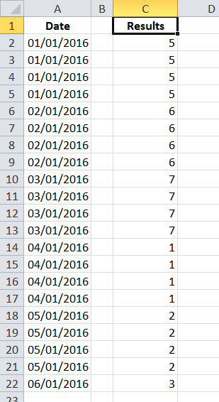
Point the WEEKDAY function at a date and it will return a number from 1 thru 7 indicating what day of the week the date is. In this case the formula reads =weekday(A2,2)

The 2 in the above formula is the return type, and here indicates that the week starts on Monday. This means that Saturday and Sunday will return values of 6 & 7.

This is perfect for using with conditional formatting.

If I plug the following formula into the conditional formatting dialog box
=(WEEKDAY(A2,2))>5

I am testing for values above 5, namely the weekend. So I can use this to put a colour fill in those dates so that they stand out.

Weekday function with Conditional Formatting

Obviously, the Results column isn’t needed because the formula is actually residing in the Edit Formatting Rule dialog box.

This is the second post discussing using Conditional formatting with a Social Media spreadsheet. Check out this previous post for another example of using conditional formatting.


This post is originally from 2016. If you want help with the newest and classic features in Excel drop me a line at catharine@mytechgenie.ca

Excel: Sequential Dates in Multiples

The Fill Series Dialog

When I’m setting up my Social Media spreadsheet in Excel, I like to limit the number of scheduled Facebook entries per day. Over time, I’ve come to think that 4 Facebook entries per day is a reasonable maximum. This lets the librarian post “live” when things are happening in the library without clogging up our follower’s feeds.

So I want to create a column of dates that looks like this:

Each date is repeated 4 times

The quickest way to do this with minimal typing is to use the Fill Series dialog box. Since Excel 2007, you can find it under the Fill menu on the  Home tab.

Finding the Fill Series Dialog

To use the Fill Series dialog, select the range of cells you want your dates to be entered in. Make sure the first cell in the range has the starting date. Then select the  Fill button and choose Series .

The Fill Series Dialog

Enter a  Step value. In this case, because I want 4 repeats of each date I’m using .25 as the Step value. If I wanted 5 repeats, I’d use .20 (and so on).

If you don’t feel like calculating how many cells to select when doing this for a date range that spans a couple of months; try using a  Stop value . With a  Stop Value, the series will stop at the first instance of the date entered into the field. Otherwise, the series will fill the entire selected range. ( In the picture above the full date is not displayed in the field, it was actually 06/01/2016.) Using a <em><strong>Stop Value</strong> </em>allows you to make a rough selection (say 500 cells) and Excel will stop when the series runs its’ course.


This post is originally from 2016, however Filling a series is still as useful in 2020 as it was then.

If you want help with the newest and classic features in Excel drop me a line at catharine@mytechgenie.ca