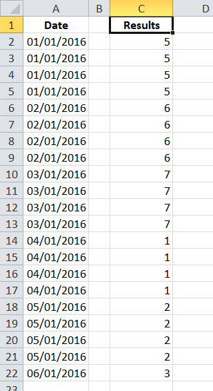
In a previous post I showed how I entered a column of repeating dates when building my Social Media spreadsheet. The next thing I like to do, is colour code those dates so that I can see at a glance when the weekend dates are. For this I use the WEEKDAY function in Excel.

Point the WEEKDAY function at a date and it will return a number from 1 thru 7 indicating what day of the week the date is. In this case the formula reads =weekday(A2,2)
The 2 in the above formula is the return type, and here indicates that the week starts on Monday. This means that Saturday and Sunday will return values of 6 & 7.
This is perfect for using with conditional formatting.
If I plug the following formula into the conditional formatting dialog box
=(WEEKDAY(A2,2))>5
I am testing for values above 5, namely the weekend. So I can use this to put a colour fill in those dates so that they stand out.

Obviously, the Results column isn’t needed because the formula is actually residing in the Edit Formatting Rule dialog box.
This is the second post discussing using Conditional formatting with a Social Media spreadsheet. Check out this previous post for another example of using conditional formatting.
This post is originally from 2016. If you want help with the newest and classic features in Excel drop me a line at catharine@mytechgenie.ca

