Home On The Range

Sometimes, when you’re teaching, its not about the complexity of the subject. Sometimes its a very simple piece of information that students get the most “mileage” out of.

When I’m teaching students MS Excel, the simplest thing that I teach them about is Named Ranges. Its the simplest thing to talk about, but the uses for ranges go on and on.

Excel Spreadsheet Example
A plain spreadsheet.

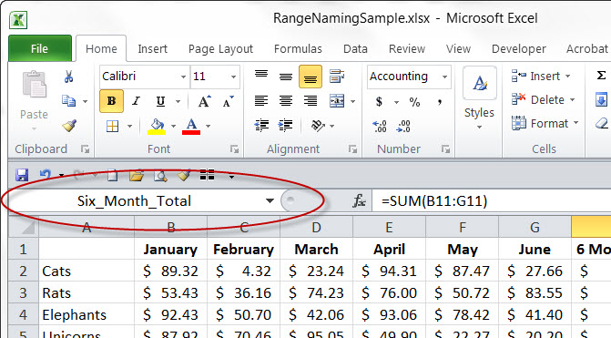
Above you see a standard Excel spreadsheet. Adding a range name or two (or ten) can help make it much easier to work with.

Adding a Range name to the Cell Address box.
Type the range name into the Cell Address box. Press Enter when done.

A range name can refer to a single cell or a group of cells, here I’ve selected the cell containing the total for the six month period (H11).

Click into the Cell address box (circled in red) and type in the desired name. There are some simple rules about naming ranges; the name can’t start with a number, can’t look like a cell reference (imagine how confusing that would be) and can’t use spaces and special characters (notice I’ve used an underscore to separate words). But after that it is up to you, to make your range name meaningful.

Adding a range name to a group of cells
Adding a range name to a group of cells.

If you are going to add a range name to a group of cells, select them and type the name into the cell address box. The most frequent mistake students make at this point, is that they forget to press the Enter key to confirm the range name.

Now, how do you use these range names?

Navigating your spreadsheet using range names.

First, you can quickly jump to your named ranges by using the drop-down menu. When you click on the drop-down menu in the cell address box, you’ll see a list of all the ranges you’ve added to your spreadsheet. Regardless of what sheet they are on. So you can use this to quickly jump to those cells that you work with again and again.

Range Names can replace cell references in formulas
Range Names can replace cell references in formulas.

Second, you can replace cell references in a formula with range names. Does =SUM(January) seem easier to read and understand than =SUM(B2:B10)? Then a formula that uses range names will make your spreadsheets easier to read.

Third, you can use range names in conjunction with all sorts of other Excel tools. As an example, try using range names with the Data Validation tool.

A Named Range provides the source for this data validation list.

In the sample above, a range name provides the source list for a drop-down list.

Data Validation Result

Resulting in this drop-down list. The list will update as the list of animals changes on Sheet1.

This is a more elegant solution for using drop-down lists, since it means your source lists can be kept on another sheet, and not clutter up the working area. This is something that is impossible to do, without using a range name.

So faster navigation, easy to read formulas and access to more powerful features in Excel. What’s not to love about range names?


Looking to make a powerful spreadsheet or do you want me to make it for you? Drop me a line at catharine@mytechgenie.ca

Social Media Spreadsheet – Conditional Formatting

I’m a big fan of Excel’s conditional formatting feature. I use it a lot in my spreadsheets to check on the quality of data, find errors and many other tasks. Here is the first of a couple of examples of how I’m using conditional formatting in my social media spreadsheet.

Just a bit of background on the spreadsheet. I use this spreadsheet to compose Facebook Posts and Tweets for the Redcliff Library. I also use it to schedule when the posts/tweets will be published. This allows me to sit down and plan a coherent sequence of posts/tweets.

I often take the Facebook posts and cut them down to shorter lengths and reuse them on Twitter. Twitter has a character limit of 140 characters. However, I don’t want to use all 140 characters if I can avoid it. Its’ generally recognized that the ideal tweet length is around 120 characters. This length allows others to retweet and add hashtags without having to edit the tweet.

So I have created 4 conditional formatting rules to help me meet this length limit.

  1. The background of the cell turns bright red [STOP] if the tweet is over 140 characters.
  2. The background of the cell turns dull red if the tweet is over 135 characters.
  3. The background of the cell turns bright orange [WARNING] if the tweet is over 125 characters.
  4. The background of the cell turns dull orange if the tweet is over 120 characters.

Why four rules? I could use 2 warnings only; at 120 and 140 characters respectively. In fact, that is where I started. But, writing tweets can be a tricky thing and I found I needed a little wiggle room to help me when I compose. The other thing to keep in mind is that the conditional format isn’t applied until I finish editing the cell (by pressing the Enter key or the checkmark). It is possible to have an interactive format applied using VBA, but those functions are memory intensive and slow down the whole spreadsheet. Since my writing process seems to involve a lot of pauses to think, stopping to apply the conditional format isn’t really a big problem for me.

So what does it look like in action?

Conditional Formatting Results

As a result, I can quickly identify which tweets need to be edited. Here are the 4 rules as displayed in the Conditional Formatting Dialog box.Conditional Formatting Dialog

These are formula based conditional formats.

closer look at formula
The formula the conditional format is based on.


A conditional formatting formula must return a value of TRUE in order to fire. The following formula uses the AND, SEARCH and LEN functions

=AND(((SEARCH(“TW”,B1))>0),LEN(H1)>140)

If you were reading this formula in something like english it would read: “If the letters TW appear in column B AND the length of text in this cell is more that 140 characters the result equals TRUE”.

Why am I testing for the presence of TW in the subject column? Remember I said that I had both Facebook and Twitter posts in the same spreadsheet. I don’t want the conditional formatting to flag Facebook posts, which by their nature are longer.

Pro Tip:

When you are writing a formula for conditional formatting, do it in a cell in the spreadsheet first. The dialog for conditional formatting is really cramped and you don’t get any help features. After you are sure the formula works, you can then copy/paste it into the dialog using the Ctrl + V keyboard shortcut. Also, because I planned on apply this conditional format to the entire Description column ($H:$H). I had cell H1 selected when I built the conditional formula. That way the formula will adjust relatively to the entire column. Using absolute and relative references properly is another tricky part of building conditional formatting formulas.

applying the coloured background fill

Once I have my formula built. I can click the format button and select the background colour fill.


When I’ve built my first format successfully I can then use it for the basis of the subsequent formulas. Just changing the length of the text in the cell.

  • =AND(((SEARCH(“TW”,B1))>0),LEN(H1)>140)
  • =AND(((SEARCH(“TW”,B1))>0),LEN(H1)>135)
  • =AND(((SEARCH(“TW”,B1))>0),LEN(H1)>125)
  • =AND(((SEARCH(“TW”,B1))>0),LEN(H1)>120)
The order of the rules and the stop if true flags must be set.

To make this really successful, the rules need to be placed in the proper order, with the Stop If True flags turned on. Now excel will check to see if the text exceeds 140 characters first, then 135, then 125 and finally 120. The Stop if True flag doesn’t need to be set on the final rule, because no other rules follow it.

Conditional formats can take time to build, but are extremely useful in many ways.


This post was originally published in 2015, and although the rules surrounding the length of a tweet have changed; my social media spreadsheet keeps chugging along. That is one of the things about a great spreadsheet. If you take the time to build it right, it will serve you well for years to come. Do you have a job that could be made easier with a well-designed spreadsheet? Drop me a line at catharine@mytechgenie.ca and let’s talk.