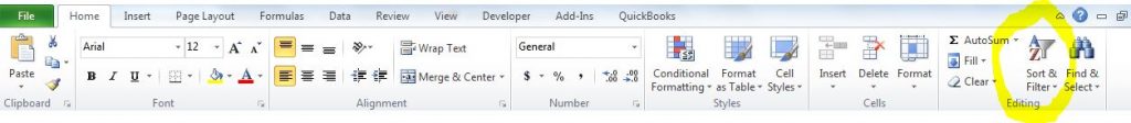
Since Excel 2007, the Filter tool has been on the Home ribbon, under the Sort and Filterdrop-down. The Filter tool can be applied to any spreadsheet where every row is a new record. Excels’ guesses about what and how to filter will be more accurate if the data has a header row. Your (human) life will be easier if you give that row a little formatting to make it stand out from the data.
If your data has gaps, select all the data (including the header row) and apply the filter. Once the filter has been applied, little triangles will appear beside each header label.
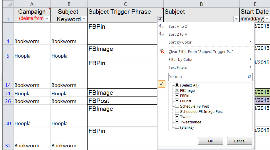
Filtering Drop-Down panel
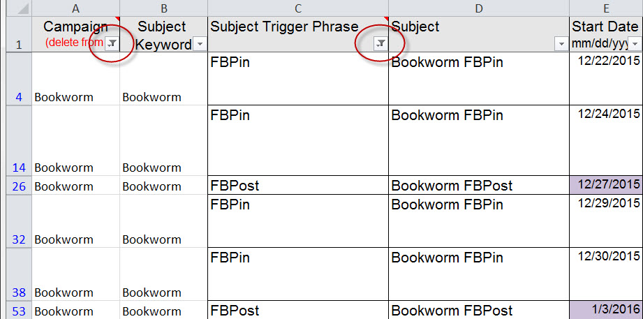
Now you can use each header to filter the data. Click on the filter drop-down and the panel will open as you can see in the picture above. Clear the check boxes beside the entries you don’t want to see. Then click the OKbutton. You can spot filtered data, because the row headers will be bright blue (and row numbers will be missing as data is filtered out). The columns where filtering is applied will have a filter icon (circled in red in the picture).
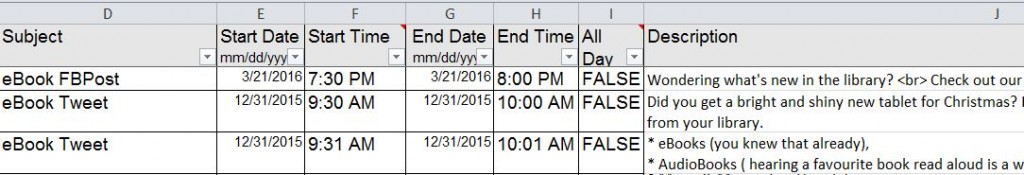
Filtering Applied
Once the filters are in place, I can filter out blanks or filter blanks in to find openings in our social media schedule. I can quickly look for Posts and Tweets with images, to ensure the image information is present. I can filter down to a single subject. All of these filters make managing my posting schedule MUCH easier.
This post is originally from 2016. If you want help with the newest and classic features in Excel drop me a line at catharine@mytechgenie.ca
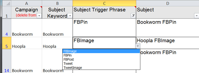
When building my Social Media spreadsheet, I want to enter my subject keywords and trigger keywords consistently. Minor typos can make it difficult to find all the relevant posts and worse; prevent scheduled posts, tweets and pins from being published on time. This is why I find the Data Validation feature in Excel so useful. As you can see in the picture above, once Data Validation is in action, my data entry is restricted to a preset list of options.
Find the Data Validation tool on the Data ribbon
Since Excel 2007, the Data Validation tool has been on the Data Ribbon. Simply select the cells you want to apply Data Validation to and press the Data Validationbutton and select Data Validation. Then the Data Validation Settingsdialogue box will appear.
Data Validation Settings
To keep the active sheet “clean”, I use a named range on another sheet as my data source (I’ve talked about that previously). Here you can see it’s called PostTypes. But you can enter short lists directly into the Source box:
Data Validation Settings
However, I find in the long run (especially for long lists) keeping the list source on another sheet makes maintenance easier.
This post is originally from 2016. If you want help with the newest and classic features in Excel drop me a line at catharine@mytechgenie.ca
As I’ve worked more with scheduling posts, tweets and pins, I’m trying to make the most of the Subject line used by Google Calendar.
Google Calendar Subject line
I’ve found that if I combine a meaningful keyword describing the post(or tweet, or pin) plus the phrase that triggers the IFTTT action, then managing the scheduled posts once they are uploaded into Google Calendar is a bit easier. It also makes it easier when I’m filtering and managing the spreadsheet too.
In my spreadsheet I use a separate column each for subject keyword and for subject trigger phrases (actually I’m paring those down to keywords too). But I want them joined together to create the actual subjects. To do this, I use the Excel CONCATENATION function. Which is most simply represented by the & symbol. In the example at the beginning of the post you can see the formula:
=B103& ” ” &C103
In this case I’m using the & symbol to join the values of cells B103 and C103 together with the string ” ” in the middle to create a nice space between words. This allows the subject phrase to be created automatically once I’ve selected the subject and trigger keywords.
This post is originally from 2016. If you want help with the newest and classic features in Excel drop me a line at catharine@mytechgenie.ca
In my Social Media spreadsheet I want to add 30 minutes to the starting time for the post. Why 30 minutes? That’s the default scheduling time in Google Calendar.
To do this, I use the TIME function. The TIME function has 3 arguments; hour, minute and seconds – all three arguments are required. So my formula would look something like this:
=F2+TIME(0,30,0)
So, I’m adding 30 minutes to the value from cell F2. Easy!
This post is originally from 2016. If you want help with the newest and classic features in Excel drop me a line at catharine@mytechgenie.ca
I’m currently advertising for an Assistant TechGenie, so unsurprisingly there are a ton of email responses hitting my email box (what is surprising; how few are from Canadian Citizens).
After I’ve sorted out the responses into a folder of likely candidates, I want to create a list of names and email addresses that I can refer to as I move through the process. The question – is there a quick way to do this from Outlook?
The answer is yes, once you build yourself a custom view. If you haven’t played with custom views in Outlook, you really should take a moment to appreciate the simple way they can add productivity to your email tasks. Today, I’m at a machine using Outlook 2016, so you might find older versions of Outlook a little different.
Create a Table View
Outlook supports numerous types of views but for this task, I’m using Table View as I can then copy and paste the information directly into a spreadsheet.
go the the Viewribbon
Click the Change Viewbutton
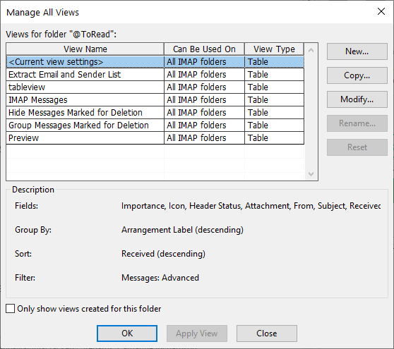
Select Manage Views, the Manage All Viewsdialog box will appear
Manage All Views
Click on the Newbutton, and the Create a New Viewdialog box will appear
Create a New Outlook View
Name your view with a meaningful name, since you will want to reuse it. Make sure Table view is selected, and make it available to all your folders. Click OK. If you are following along, at this point you will notice that I have already removed the columns I don’t want.
Remove all the columns except the ones you plan on using
But there is one column I do want – the sender’s email address. And you will not find it in the lists of available columns. Instead, try this trick I picked up from espacecode.com
Add a Custom Column
Use the New Columnbutton, the New Columndialog will appear.
Name the column (the name can not be “email”).
From the Typedrop down list, choose Formula.
Paste the following formula into the Formulafield:
Click on the OKbutton to complete this step and the Advanced View Settings: Your View Name will appear
The Advanced View Settings Dialog
Fine tune your View
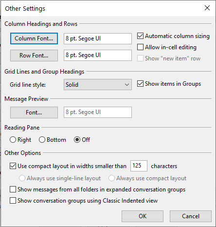
Click the Other Settingsbutton and the Other Settings dialog will appear
The Other Settings dialog box
Make sure that the Reading Paneis turned off as well.
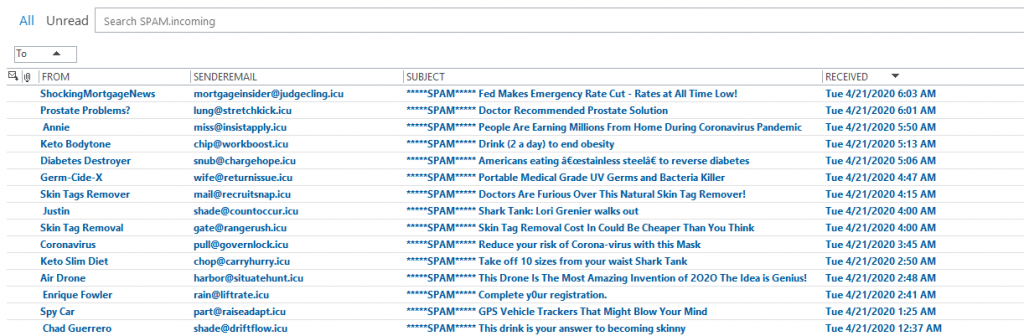
Click on the OKbutton twice to return to the folder view. If you have Message Previewsturned on for this folder, turn them off. The result should look as follows:
Here are the email addresses of spammers exposed.
Using Your Custom View
You can now copy this information directly into a spreadsheet and easily make a list of names and email addresses. And since this is a named view, when the task is done and I want to return to my preferred email view, I can do so. But I can reapply the view at any time.
Are you looking for methods to handle your email overload? Drop ME an email catharine@mytechgenie.ca and we can build some simple tools (like this one) to help you manage your email more effectively.
Join me in this webinar, hosted by the Medicine Hat Chamber of Commerce
There’s been a lot of talk lately about “Zoom Fatigue”. The trailer above is one way to combat fatigue. Creating trailers for your presentations allow you to shorten the presentation by introducing information ahead of time. Like a movie trailer; your talk trailer tells your audience what to expect and allows you to cut your talk time down.
And why limit yourself to a single trailer? For longer and more complex materials, you might want to create multiple trailers that can prepare your audience properly for your talk.
Creating your trailer in PowerPoint allows you to easily reuse elements in future trailers. This saves time and strengthens your brand presence. You can bet I’ll be reusingthe little animated stars on this slide that act as an attention getter for keywords.
These little purple star animations pull the eye to key words
Like the idea of saving time? Drop me a line, and lets’ make something fantastic for your next presentation. A reusablesomething fantastic!
The latest version of PowerPoint allows you to export your presentation as an animated GIF. Animated GIFs are great for catching the eye on social media.
Redcliff Library Board Member Promotion – as an animated GIF
There are of course, lots of animated GIF sofware packages available, many are free. But none are as useful as PowerPoint when it comes to incorporating imagery that you already have on hand. Remember to keep the size of the file down, as Twitter limits animated GIF size to 5MB.
If you want a little more room or sound, remember that you can export your PowerPoint presentation as a video in mp4 format.
You notice some differences between the video and GIF versions of this little social media piece. This is to optimize file size for the animated GIF.
The beauty of creating this in PowerPoint is that it is easily accessible for updating by the client.
Like what you see? Drop me a line, and lets’ make something fantastic for your next social media promotion. A reusablesomething fantastic!
Music:
Path Of The Fireflies by AERØHEAD | https://soundcloud.com/aerohead
Music promoted by https://www.free-stock-music.com