A little bit of history – lost … and found

Excel has been around for decades, so it isn’t surprising that there are many features tucked away under the hood. What is surprising is when a useful feature is lost and only careful archeology can bring it back to life.

Excel 4.0 had a rudimentary macro language, mostly using excel formula approaches to building functionality. This was replaced by the VBA programming language. But there are still useful little items tucked away in this early language that haven’t been replaced.

One of these is Get.Cell.

Get.Cell had a boatload of switches that allowed the user to pull information about the cell formatting and contents and most of these have been replaced by the Cell and Type functions in Excel.

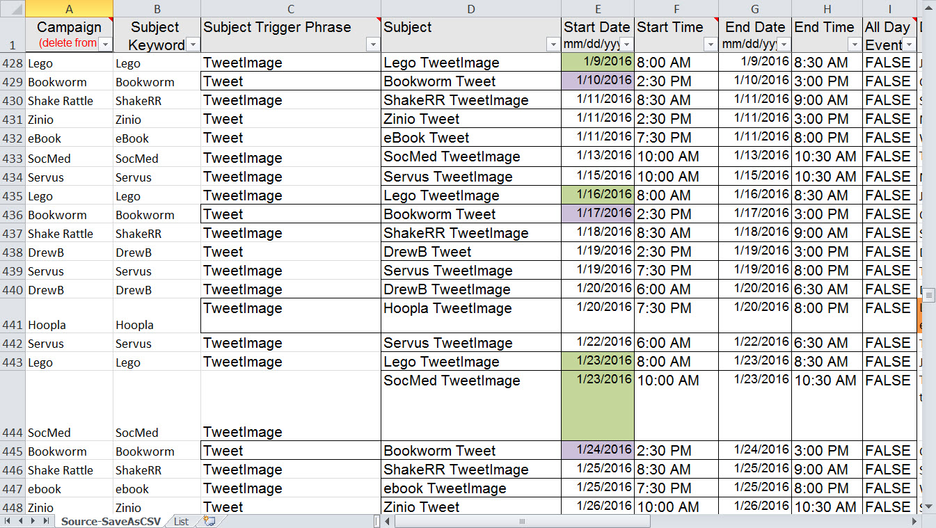
But one piece of information that Cell and Type can’t tell you is whether your cell or cells contain formulas vs values and sometimes this is a very handy thing to know at a glance. For example, if you build a spreadsheet using formulas to estimate amounts; but then start to drop in values as more concrete information becomes available.

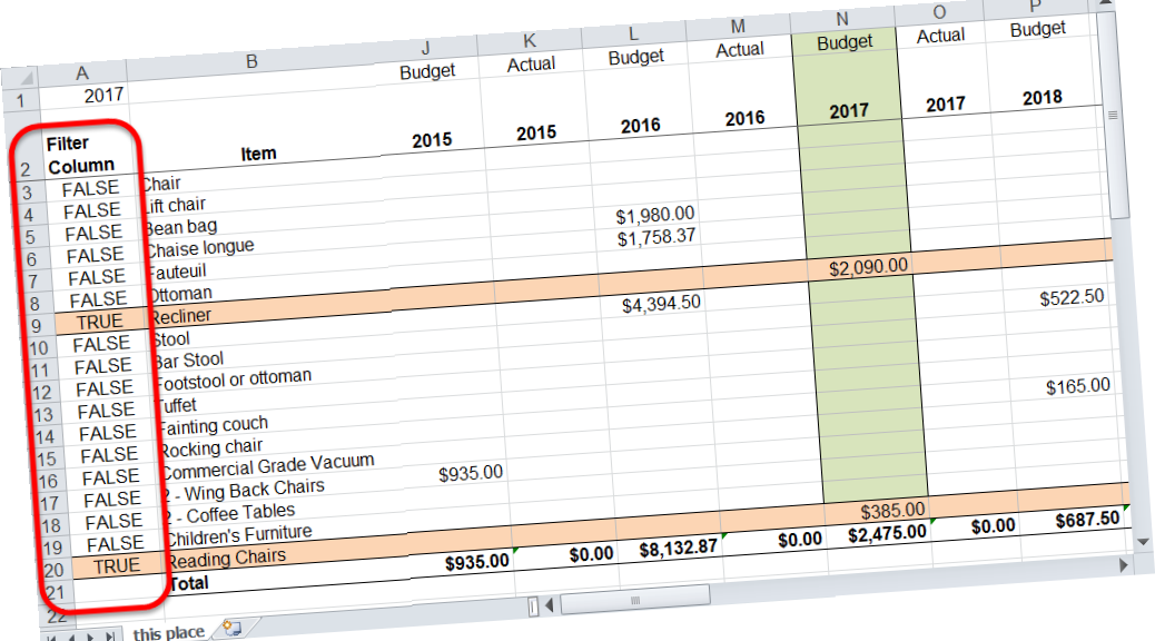
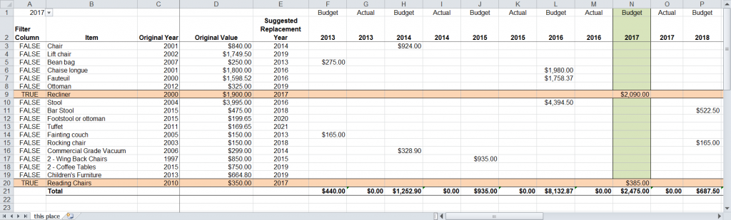
In this situation I like to format cells containing formulas differently from the cells containing values, so that I can see at a glance where my estimates are. Its’ handy to have the formatting change automatically, so I don’t have to remember what my rules are weeks or months later.

This is where Get.Cell shines. The syntax I’m going to use is

=GET.CELL(48,A1) – where A1 is the cell I’m going to reference.

The trick here is that Get.Cell is NOT entered in a cell, but instead as a named formula. After creating the named formula, I can reference it while applying conditional formatting. In this way, when the type of content in the cell changes the conditional formatting automatically updates.

Where does one find information about the Get.Cell function? Not from Microsoft or at least not easily from Microsoft.

Try this post https://www.mrexcel.com/forum/excel-questions/20611-info-only-get-cell-arguments.html to see the possible switches for Get.Cell

First published in 2017, the Get.Cell function remains useful today. I remain hopeful that MS will incorporate its’ functionality in newer versions of Excel. If you want expertise in Excel, drop me a line at catharine@mytechgenie.ca

July 13, 2022July 6, 2022

Highlighting the Current Year

Here is a version of a spreadsheet that I’ve been using for a couple of years to track and plan capital purchases. A number of people review this spreadsheet and I want to make it as easy as possible for them to read the spreadsheet. You’ll notice that the Budget year is highlighted in green and items being purchased in that year are highlighted as well. This is accomplished with our friend conditional formatting and the following spreadsheet functions:

ADDRESS
ROW
COLUMN
MATCH
INDIRECT
ISBLANK

Spreadsheet with automatic highlighting — Capital Budget Spreadsheet – note the row and column (year) highlights

This spreadsheet makes use of a helper column of formulas. Rows where the value equals TRUE are highlighted.

Cells give a value of TRUE when there is a value for that row in the Budget Year selected in cell A1. You can see that 2017 has been selected as the Budget Year and that rows 9 and 20 have a value for that year and are highlighted as a result.

This is the formula that returns the value

=ISBLANK(INDIRECT(ADDRESS(ROW(),MATCH($A$1,$F$2:$AU$2,0)+5,3,TRUE)))=FALSE

Working from the interior of the formula outward.

MATCH($A$1,$F$2:$AU$2,0)

This looks for a match between the value in A1 and the Budget year headings which start in cell F2 and go to AU2 (the year 2033, which is incredibly optimistic – but that is another story). MATCH returns the number of the first item in that array of cells that matches the value in A1. This is why even though there are two columns for every year (a Budget column and an Actual column) MATCH will only return the Budget column, as it is the first value to match.

So the result of MATCH($A$1,$F$2:$AU$2,0) is 9

However, if I actually want to capture the column I need to to add 5 to compensate for the fact I have 5 columns (A-E) before column F and the year headings begin. This is why I’m adding 5 in the formula.

MATCH($A$1,$F$2:$AU$2,0)+5 =14

In the next step I use ADDRESS and ROW to capture the address of the cell I’m testing.

ADDRESS(ROW(),14,3,TRUE))

ROW() captures the value of the row of the cell where the formula is written. If the formula is in A3, then row() returns 3.

ADDRESS turns the cell address of the referenced cell (not its’ contents). In our example; ADDRESS(3,14,3,TRUE)=”$N3″

The ISBLANK function in the next step has a bit of a hiccup with that “$N3” string, so we use INDIRECT to convert that string to something ISBLANK can understand.

Finally, ISBLANK is used to test if there is a value in the referenced cell or not. If there is nothing in the cell ISBLANK = TRUE.

If ISBLANK = TRUE, then the last portion of the formula looks like this: TRUE does not equal FALSE, so the result of the formula in cell A3 is FALSE.

I could have put that formula into the conditional formatting dialogue – but for clarity and ease of working I choose to make the helper column instead.

In the conditional formatting dialogue I’ve used the following formula =$A3=TRUE

I’m using a simpler version of the formula in the conditional formatting dialogue to highlight the year.

=MATCH($A1,$F$2:$AU$2,0)+5=COLUMN()

In this case I find the column number of the year and test to see if it matches the column number of the current cell. If it does then the cell receives a green highlight fill.

Cell A1 uses Data Validation to offer the user a nice drop-down list of years.

This post is from 2017. The technique is still valid and very useful! If you want help with the newest and classic features in Excel drop me a line at catharine@mytechgenie.ca

July 8, 2022July 6, 2022

Making Powerful Image Quotes

For those of you who haven’t had one of my seminars on using PowerPoint to create powerful image quotes for your social media feed; now’s the time to get out into the garden with your camera phone and take a few photos.

You need to create a stockpile of good background photos that you can use for fresh quotes. And summertime in your garden is a great time and place to do this.

Closeups of plants and flowers make a great background for a variety of quotes – like this one I found on the Olds Municipal Library Facebook feed.

You can see how they use a transparent overlay over part of the picture to help the text stand out.

You may not have an immediate need for those pictures, but you can set them aside for later use, like this image of purple pink chrysanthemums (my chrysanthemums are looking particularly lovely this year, due to the fact I’ve just bought them).

You know you’re in love when you can’t fall asleep because reality is finally better than your dreams.” ― Dr. Seuss The colour of these flowers, will do nicely for a different Valentines’ Day image quote.

You don’t need a fancy camera to get these pictures, the camera on your phone will do just fine. But do make sure you take your pictures in both horizontal and vertical orientations to make sure you have more layout options later on.

When you don’t know how you’ll be using those photos, options are very good.

Don’t just focus on flowers (hehe, see what I did there), leaves and foliage are useful too.

Don’t forget that the same picture can be used multiple ways, once you start throwing colour filters and special effects at it.

Left is original photo – the right has the saturation cranked up.

Oh, and that image has been flipped, since I like the leaves appearing on the left side of the photo better.

A final tip, when saving your image quotes, use the PNG format, it creates fewer artifacts (small jiggly lines that make text harder to read) than JPEG.

This post is originally from 2018. If you want help with the newest and classic features in PowerPoint drop me a line at catharine@mytechgenie.ca

July 6, 2022

PowerPoint – Making a Mask

Creating a mask effect in PowerPoint is easy, once you’ve located the Shape Combine command. You can add this command to the Ribbon or the Quick Access Toolbar.

Below, you see it being added to my toolbar.

Adding the Shape Combine Command to the Toolbar, alternately look for the Combine Shapes command as more options are available.The command will not be active until there are two shapes selected. Below, I’ve created a blue rectangle and a red oval. The oval shape will be cut out from the rectangle.

Blue rectangle with red oval positioned for the cut out. You may prefer to add the Combine Shapes command instead. More options are available as you can see below.

The result of the Shape Combine command, a rectangle with an oval “hole: in the center.

The result of the Combine Shapes CommandOnce the mask is created, you can dress it up. Below, I’ve changed the fill to an image of a leafy forest floor.

The forest floor has a hole in it. Now I can layer whatever image I wish (in this case a frog) under the mask. You can animate the layer underneath the mask. Can you image a wheel of creatures rotating into the viewpoint in the center of the mask? That would be great for a talk about ecology!

This post is originally from 2016. If you want help with the newest and classic features in PowerPoint drop me a line at catharine@mytechgenie.ca
Frog image via Wikipedia

June 7, 2022June 3, 2022

Making Lace Photos

Lace

In the last post, I showed how to turn a photo into a stencil. This time, we’ll be adding a lace effect to this photo.

A Wedding Kiss photo — Wedding Kiss – Courtesy Pixabay and Peter Klaus

Using this photo:

Close up of a Chrysanthemum — Chrysanthemum from Windows 10 default photo set

After inserting the photo and changing the background colour, go to Picture Tools>Format>Picture Corrections. Set Sharpness to 100%. The picture may look worse at this point, but don’t worry.

The photo has had Sharpness applied to the maximum

Now, set Contrast to 100%. Yep, it definitely looks worse.

Select Picture Color and adjust Saturation to 0%

Things are looking up again. Select Picture Tools>Format>Color>Set Transparent Color. Click on a black portion of the picture.

Now is the time for a little cropping and copying that will make the lace effect stand out.

Cropping and mirroring the photo, makes it look more “lace like”

And finally, layer the lace over the Wedding Kiss photo for the result.

This post is originally from 2018. If you want help with the newest and classic features in PowerPoint drop me a line at catharine@mytechgenie.ca

June 3, 2022June 3, 2022

Photo Stencils

Duotone photos are the current thing online and you can buy software or use a service to convert your photos into duotone photos. But did you know that you can easily create duotone photos in PowerPoint?

Along the way to this technique, I’ll show you how to make stencils and lace out of your photos as well.

Stencils

I’m going to use this photo of penguins to make a stencil type image. I’m using Office 365, but this can be done in PowerPoint 2010 as well. I’ve also changed the background colour of my slides. This isn’t necessary, but will make the images easier to understand.

After inserting the photo and changing the background colour, go to Picture Tools>Format>Artistic Effects. You can use either the Photocopy effect or the Cutout effect. The main difference will be the amount of small detail retained by the photo. I like the Cutout option with this photo.

Picture of penguins with Cutout Effect applied — The first step in creating a stencil, applying the Cutout Effect

Reduce the number of shades to 1

The Cutout now has a the number of shades reduced to zero

Select Picture Corrections and adjust Contrast to 100%

Select Picture Color and adjust Saturation to 0%

Saturation on the picture is now set to zero, removing the small blue highlights that were visible before.

Even if you are on Office 365, you’ll need to use the Ribbon. The Set Transparent Color command is not on the Picture Color Tab. Select Picture Tools>Format>Color>Set Transparent Color. Click on a black portion of the picture. Voila! A stencil of Penguins that takes on the colour of the slide background.

After the black portions of the picture have been removed, the slide background is visible.

You can use a variation on this technique to make a “lace” overlay.

This post is originally from 2018 If you want help with the newest and classic features in PowerPoint drop me a line at catharine@mytechgenie.ca

December 17, 2021July 31, 2021

Excel: Frozen

Freezing panes is a basic tool to make a large spreadsheet easier to work with. In my social media spreadsheet I like to freeze the header row into position. Then no matter how far I scroll down the sheet, the columns are labelled.

To turn on frozen panes, select the cell below the row & column you wish to freeze into position. Since I don’t want to freeze any columns, I select cell A2.

Freezing Panes using the Active Cell position" width — Freezing Panes using the Active Cell position” width

Select the View Ribbon, Click on the Freeze Panes button, and choose Freeze Panes (or Freeze Top Row in this scenario).

Now you can scroll for hundreds of rows, and each column is nicely labelled – no guessing!

This post is originally from 2016. If you want help with the newest and classic features in Excel drop me a line at catharine@mytechgenie.ca

November 10, 2021July 31, 2021

Excel: Select Visible (1)

I built my Social Media spreadsheet in an Excel spreadsheet with all the tools I want built in (formulas, conditional formatting and data validation). Ultimately, I will transfer my information into a stripped down spreadsheet in csv (comma separated) format. This is the format that Google Calendars will accept.

When I transfer my posts to this spreadsheet, I don’t want to include any blank rows AND I only want to copy and paste once. How do I perform this little piece of magic? I use the Excel command for selecting visible cells only.

Go To Special Dialog, select Visible cells only

Tucked away in the Go To Special dialog is the option for selecting only the visible cells in a region. This takes what could be multiple copy/paste operations and condenses them into one step.

First filter your data so that blanks do not appear, then press the F5 function key to bring up the Go To dialog box.

Press the Special button to open the Go To Special dialog box, choose Visible cells only and press OK. Now when you copy the selected cells, only the cells you can see are copied.

In my next post I’ll show the method to put this useful button on your Quick Access Toolbar.

This post is originally from 2016. If you want help with the newest and classic features in Excel drop me a line at catharine@mytechgenie.ca