You’re working on a research project, and you’ve dug through the bowels of the internet to find some information that is relevant to your question. After a brief interlude of looking up which artist sang the song you have stuck in your head in a new tab, your caffeine-saturated finger muscles accidentally press the close button/Ctrl + W one too many times. Oh no! We’ve all been there, but not all of us know what to do about it. Until now.
Press Ctrl + Shift + T to reopen the tab you’ve just closed, and the tab you closed before that, and so on. What’s more, if your computer updated overnight and closed your browser, you can use this same trick after you open your browser back up to recall all the tabs that you lost. This trick works in every browser on Windows 10.
Another day at work, and your boss is checking in to see what you’ve accomplished. Of the several windows you have open, both for the project and for reference, one has very small text, and another has a font colour that doesn’t stand out against the background. How can you show your boss your progress without them having to squint 6 inches away from your screen? Or perhaps you’re presenting an Excel spreadsheet to a huge room. How can you make sure the people at the back can see the values in the cells?
Windows 10’s magnifier shortcut is your easy accommodation for this problem. By pressing Windows Logo Key + = (equals), you can zoom your screen in on wherever your cursor sits. This shortcut comes in three versions. In Full Screen Version (Ctrl + Alt + F), the entire screen zooms in on your cursor. In Lens Version ( Ctrl + Alt + L), a small window showing the magnified area appears. In Docked Version (Ctrl + Alt + D), the magnified area is displayed in a wide panel that appears at the top of the screen. These versions can be cycled between using Ctrl + Alt + M. In all three versions, the area magnified changes depending on where you move your mouse, and each version is also accompanied by a miniature window which allows you to:
Change the degree of magnification
Access a text-to-speech feature
Change the speed and accent of the text-to-speech feature*
Exit the magnifier by pressing Windows Logo Key + Esc.
Imagine that you’re a CSIS agent, and you’ve been asked to write up a report regarding the text messages exchanged between two suspects in a terror plot. Straightforward enough – unless the suspects use emojis. What is your senior agent going to think if your report states that one suspect used the “exploding head” emoji? Without a way to show the emojis themselves in high resolution, confusion might ensue.
Of course, you could have plenty of mundane reasons to want emojis in your documents as well. Perhaps you want your emails in Outlook to seem more approachable, or maybe you want to construct a simulated text conversation on a PowerPoint slide. Fortunately, Windows 10 has a solution: a searchable emoji keyboard. This tool can be called upon in almost any Windows 10 app by pressing the Windows Logo Key + . (period). The dialogue box that appears is the same in any app that you open it in, and has all the same emoji options that you have on your phone, as well as pre-made “kaomojis” [(づ ̄3 ̄)づ╭❤~, (❁´◡`❁), etc.]. You can keep typing in the same spot in the document to search for a specific emoji, or you can click on the dialogue box’s various category tabs to view related options.
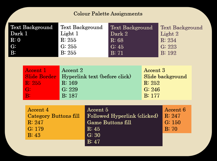
I find it useful when creating a presentation that has a custom colour palette to create a custom layout like the one below:
Colour Palette Assignment Slide Layout – accessible via Master view, or by selecting the layout
You’ll note that the RGB values for the colours are listed, and this is because prior to PowerPoint 2013, the eyedropper tool was not available. I also find it tremendously helpful to note what I use each colour for, so that when I open this file in a couple of years from now there will be a little less detective work.
This post is originally from 2018 If you want help with the newest and classic features in PowerPoint drop me a line at catharine@mytechgenie.ca
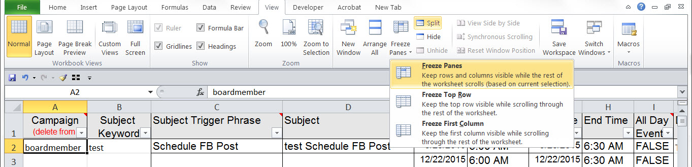
Freezing panes is a basic tool to make a large spreadsheet easier to work with. In my social media spreadsheet I like to freeze the header row into position. Then no matter how far I scroll down the sheet, the columns are labelled.
To turn on frozen panes, select the cell below the row & column you wish to freeze into position. Since I don’t want to freeze any columns, I select cell A2.
Freezing Panes using the Active Cell position” width
Select the View Ribbon, Click on the Freeze Panesbutton, and choose Freeze Panes(or Freeze Top Rowin this scenario).
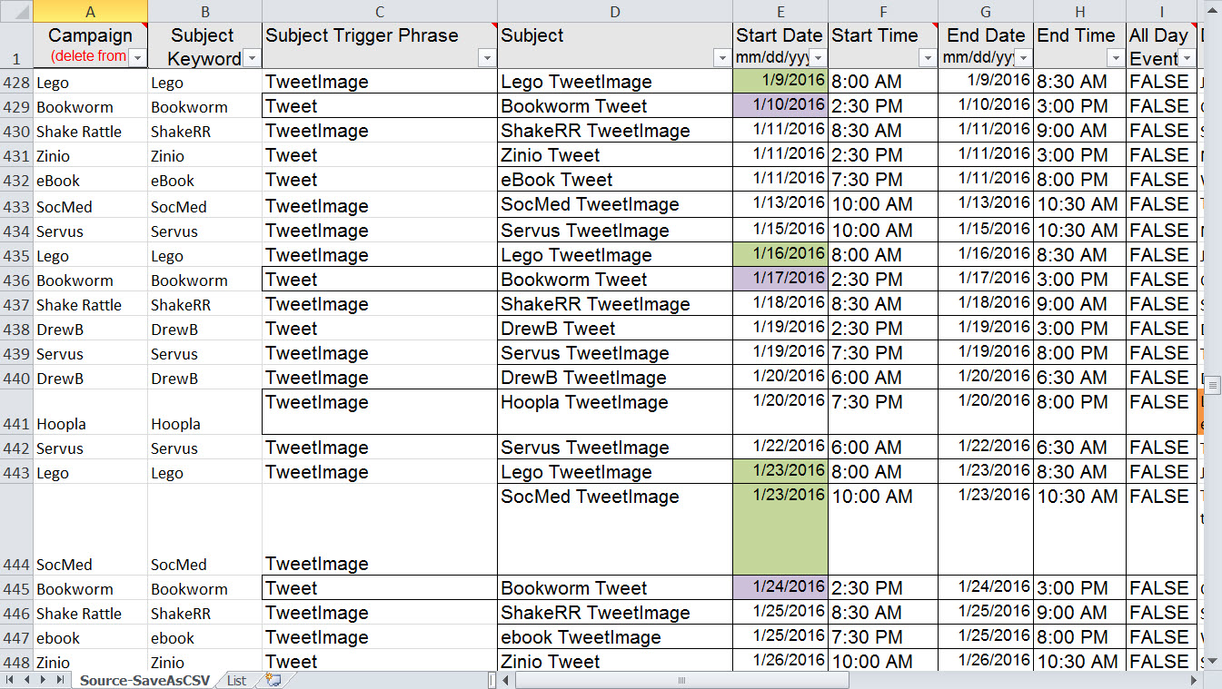
Freezing Panes Results
Now you can scroll for hundreds of rows, and each column is nicely labelled – no guessing!
This post is originally from 2016. If you want help with the newest and classic features in Excel drop me a line at catharine@mytechgenie.ca
The Select Visible Cells Only button on the Quick Access Toolbar
The Select Visible Cells Only function is so useful, I like to add it to the Quick Access Toolbar (QAT) in Excel. These instructions are based on Excel 2010, but will be similar in all current versions of Excel.
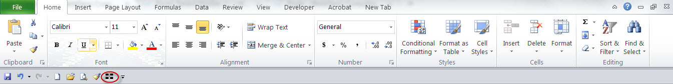
Quick Access Toolbar Customization
The Quick Access Toolbar starts in the top right corner of the Excel window. The customize button is circled in red. Clicking on that button displays the menu shown below.
Move the QAT under the ribbon
The first change I like to make is to its’ position. I like to move it under the Ribbon, since there will be more room for buttons there. Over time I tend to fill the QAT up with frequently used tools.
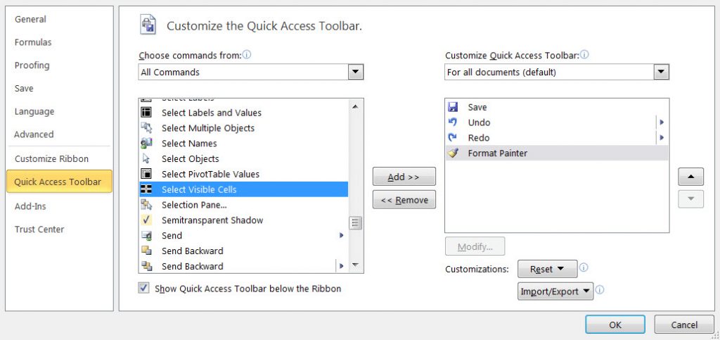
After I move the QAT below the ribbon, I go hunting for useful commands to add. Click the More Commands… option and the Customize the Quick Access Toolbardialog opens up.
Customize the Quick Access Toolbar – Popular Commands
The dialog box defaults to Popular Commands. Try scrolling through this list and find the Format Painter. Press the Addbutton, to add it to the Quick Access Toolbar. This is a useful tool to have at hand!
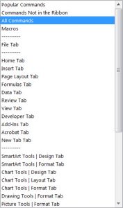
By clicking on the Choose commands fromdrop-down list, a selection will be displayed.
Drop-down list of source commands.
Select All Commandsfrom this list. Hundreds of Excel commands will display, and this is where it is useful to know the name of the command you are looking for. Scroll until you find Select Visible Cells.
Finding the Select Visible Cells command
Select it, Click on the Addbutton, and click OK.
Simply select the cells you wish to copy and press the Select Visible Cellsbutton. Paste your information and only what you see will be pasted.
This post is originally from 2016. If you want help with the newest and classic features in Excel drop me a line at catharine@mytechgenie.ca
I built my Social Media spreadsheet in an Excel spreadsheet with all the tools I want built in (formulas, conditional formatting and data validation). Ultimately, I will transfer my information into a stripped down spreadsheet in csv (comma separated) format. This is the format that Google Calendars will accept.
When I transfer my posts to this spreadsheet, I don’t want to include any blank rows AND I only want to copy and paste once. How do I perform this little piece of magic? I use the Excel command for selecting visible cells only.
Go To Special Dialog, select Visible cells only
Tucked away in the Go To Specialdialog is the option for selecting only the visible cells in a region. This takes what could be multiple copy/paste operations and condenses them into one step.
First filter your data so that blanks do not appear, then press the F5 function key to bring up the Go Todialog box.
Press the Specialbutton to open the Go To Specialdialog box, choose Visible cells onlyand press OK. Now when you copy the selected cells, only the cells you can see are copied.
In my next post I’ll show the method to put this useful button on your Quick Access Toolbar.
This post is originally from 2016. If you want help with the newest and classic features in Excel drop me a line at catharine@mytechgenie.ca
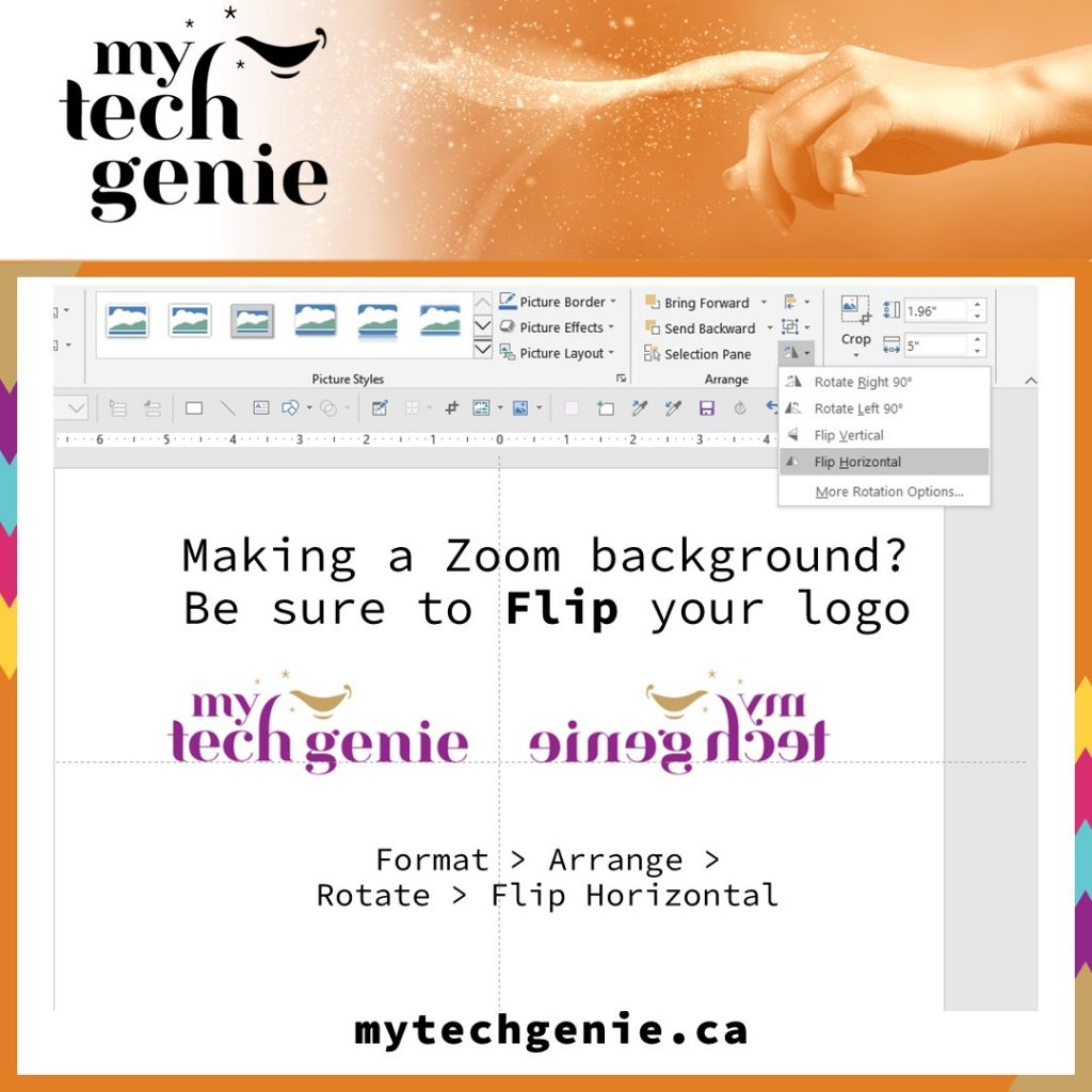
You can make a professional looking Zoom background quickly in PowerPoint. Just be sure to use a 16 x 9 dimension slide.
Oh, and flip your logo or any text on the slide. Yes, it will be mirrored. But when uploaded to Zoom as a virtual background, it will read properly for your audience.
Don’t forget to reverse images
After creating your slide, save it as a jpeg and then upload it to Zoom.
Looking for help with getting the most from your presentations?
Contact me at catharine@mytechgenie.ca
Flash Fill was introduced in 2013, but I have clients who are just upgrading to 2013 this year. This is the kind of feature that makes upgrading worthwhile.
Flash Fill is a new tool introduced in Excel 2013. Its a simple tool to handle a frequent problem. You have a small set of data and you need to break it apart into separate columns or join separate columns of data together.
Previously, I would have handled it with a series of text functions in Excel (LEFT, RIGHT, MID) combined with FIND and LEN if the data was complex enough. But if the data set is small, writing a formula sometimes seems like an overly complicated answer to a simple problem (why not just retype?).
Now Flash Fill is stepping in to help you handle this problem. If you give it a series of data (column orientation only) and an example of the pattern you want to extract, it will extract the data for you.
Flash Fill captures the first names only from the adjacent column
You can see once the second name is typed in the column adjacent to the list of full names, Flash Fill is able to see the pattern and offer all the first names in the list. Pressing enter autocompletes the action and the names are filled in. To do this, there can not be more than two blank columns between the source data and the resulting column. You can use the Ctrl + e shortcut to start flash fill.
Note the Flash Fill Icon displaying after the Ctrl + e shortcut was used.
You can click the Flash Fill icon to display the menu, accepting the suggestions will have all the names autocomplete.
The Flash Fill Menu
Here is an even trickier scenario, in the list above some names have two middle initials. Using the “default” flash fill means only the second initial will display in those names. However if I return to any of the names on the list (with two initials) and correct the example to two initials, all of the two initials examples will be extracted.
Flash Fill double initial example
I find that seriously impressive.
I can split data in a cell into multiple columns and I can also use Flash Fill to join multiple columns of data together.
Joining separate columns using Flash Fill
The same technique used above. Note that I’ve been able to add commas and periods to the text as well.
Using Flash Fill to apply formatting
In the same way, I can use Flash Fill to apply formatting, in this case putting a space between the first and second part of a postal code. You can also use it to format telephone numbers and date information.
I was (and still am) excited to share Flash Fill with my favourite clients. If you are interested in becoming one of my clients, drop me a line at catharine@mytechgenie.ca