
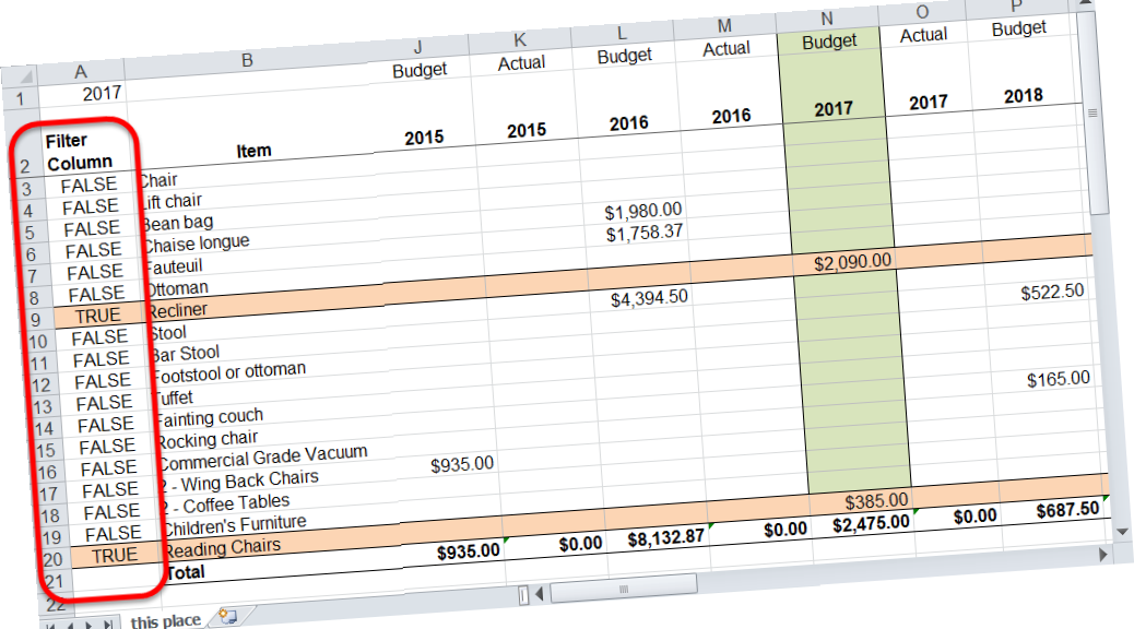
Here is a version of a spreadsheet that I’ve been using for a couple of years to track and plan capital purchases. A number of people review this spreadsheet and I want to make it as easy as possible for them to read the spreadsheet. You’ll notice that the Budget year is highlighted in green and items being purchased in that year are highlighted as well. This is accomplished with our friend conditional formatting and the following spreadsheet functions:
- ADDRESS
- ROW
- COLUMN
- MATCH
- INDIRECT
- ISBLANK
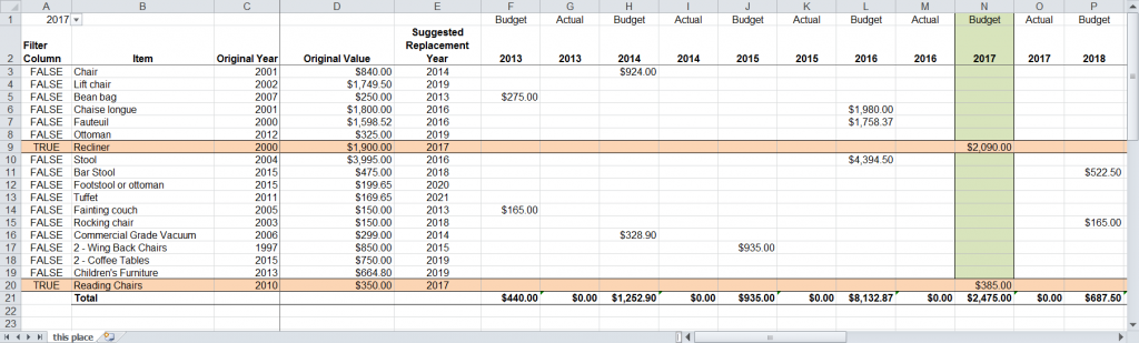
This spreadsheet makes use of a helper column of formulas. Rows where the value equals TRUE are highlighted.

Cells give a value of TRUE when there is a value for that row in the Budget Year selected in cell A1. You can see that 2017 has been selected as the Budget Year and that rows 9 and 20 have a value for that year and are highlighted as a result.
This is the formula that returns the value
=ISBLANK(INDIRECT(ADDRESS(ROW(),MATCH($A$1,$F$2:$AU$2,0)+5,3,TRUE)))=FALSE
Working from the interior of the formula outward.
MATCH($A$1,$F$2:$AU$2,0)
This looks for a match between the value in A1 and the Budget year headings which start in cell F2 and go to AU2 (the year 2033, which is incredibly optimistic – but that is another story). MATCH returns the number of the first item in that array of cells that matches the value in A1. This is why even though there are two columns for every year (a Budget column and an Actual column) MATCH will only return the Budget column, as it is the first value to match.
So the result of MATCH($A$1,$F$2:$AU$2,0) is 9
However, if I actually want to capture the column I need to to add 5 to compensate for the fact I have 5 columns (A-E) before column F and the year headings begin. This is why I’m adding 5 in the formula.
MATCH($A$1,$F$2:$AU$2,0)+5 =14
In the next step I use ADDRESS and ROW to capture the address of the cell I’m testing.
ADDRESS(ROW(),14,3,TRUE))
ROW() captures the value of the row of the cell where the formula is written. If the formula is in A3, then row() returns 3.
ADDRESS turns the cell address of the referenced cell (not its’ contents). In our example; ADDRESS(3,14,3,TRUE)=”$N3″
The ISBLANK function in the next step has a bit of a hiccup with that “$N3” string, so we use INDIRECT to convert that string to something ISBLANK can understand.
Finally, ISBLANK is used to test if there is a value in the referenced cell or not. If there is nothing in the cell ISBLANK = TRUE.
If ISBLANK = TRUE, then the last portion of the formula looks like this: TRUE does not equal FALSE, so the result of the formula in cell A3 is FALSE.
I could have put that formula into the conditional formatting dialogue – but for clarity and ease of working I choose to make the helper column instead.
In the conditional formatting dialogue I’ve used the following formula =$A3=TRUE
I’m using a simpler version of the formula in the conditional formatting dialogue to highlight the year.
=MATCH($A1,$F$2:$AU$2,0)+5=COLUMN()
In this case I find the column number of the year and test to see if it matches the column number of the current cell. If it does then the cell receives a green highlight fill.
Cell A1 uses Data Validation to offer the user a nice drop-down list of years.
This post is from 2017. The technique is still valid and very useful! If you want help with the newest and classic features in Excel drop me a line at catharine@mytechgenie.ca