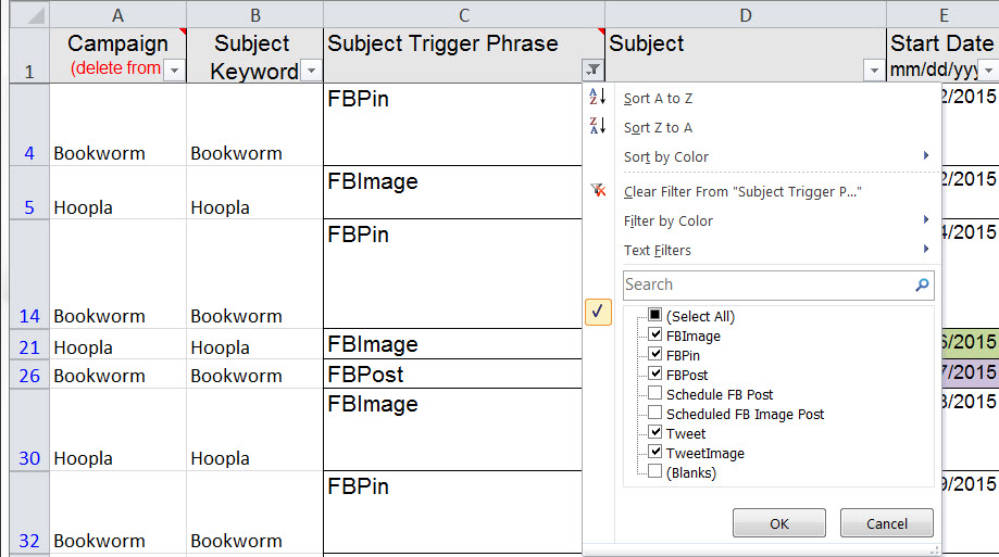
Since Excel 2007, the Filter tool has been on the Home ribbon, under the Sort and Filter drop-down. The Filter tool can be applied to any spreadsheet where every row is a new record. Excels’ guesses about what and how to filter will be more accurate if the data has a header row. Your (human) life will be easier if you give that row a little formatting to make it stand out from the data.
If your data has gaps, select all the data (including the header row) and apply the filter. Once the filter has been applied, little triangles will appear beside each header label.

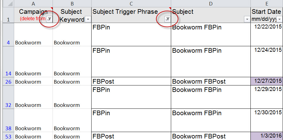
Now you can use each header to filter the data. Click on the filter drop-down and the panel will open as you can see in the picture above. Clear the check boxes beside the entries you don’t want to see. Then click the OK button. You can spot filtered data, because the row headers will be bright blue (and row numbers will be missing as data is filtered out). The columns where filtering is applied will have a filter icon (circled in red in the picture).

Once the filters are in place, I can filter out blanks or filter blanks in to find openings in our social media schedule. I can quickly look for Posts and Tweets with images, to ensure the image information is present. I can filter down to a single subject. All of these filters make managing my posting schedule MUCH easier.
This post is originally from 2016. If you want help with the newest and classic features in Excel drop me a line at catharine@mytechgenie.ca

